Loss Reserving Through Penalized Likelihood

undefined

1. Introduction

The publication marking the debut of the CAS Monograph series, Stochastic Loss Reserving Using Bayesian MCMC Models (Meyers 2019), opened the door to the practical implementation of stochastic loss reserving using a chain ladder method. The approach is built upon earlier actuarial research and literature that aims to broaden the deterministic reserving framework by incorporating reserve volatility and prediction error. Rooted in the Mack model, which first introduced a distribution-free framework for the chain ladder method to examine reserve variance, subsequent stochastic loss reserving models and methodologies have expanded in various directions by incorporating generalized linear models (GLMs) (England and Verrall 2002), bootstrap techniques for obtaining reserve distribution and prediction error estimation, and a broader compilation of alternative statistical models for comparison.

While these developments have significantly advanced stochastic reserving practice, much of the literature focuses on the application of various stochastic reserving techniques or simulation techniques rather than the underlying structure of the likelihood equations themselves that arise from the GLM. In particular, the multiplicative mean structure that underlies many stochastic reserving models gives rise to a set of balance relationships between accident-year totals and development-period totals. Examining these relationships through the lens of likelihood functions can provide useful insight into how a basic stochastic loss reserving model using GLM operates and how it extends naturally from a deterministic reserving model.

Motivated by this gap in actuarial literature, this paper first revisits stochastic loss reserving through the lens of likelihood functions. By examining the row and column likelihood equations implied by a multiplicative mean model, I show that the deterministic chain ladder estimator arises naturally as the solution to an unpenalized GLM framework. I then further explore how penalized GLMs can incorporate a priori information about development patterns and expected loss estimates, providing a natural and intuitive credibility-weighted estimation extension to the unpenalized stochastic reserving framework.

2. Chain ladder and unpenalized GLM

Suppose we have an i × j loss triangle, where i is the number of accident-year periods (rows) and j is the number of development periods (columns). England and Verrall (2002) have shown that, to a large extent, it is irrelevant whether incremental or cumulative data are used when considering claims reserving in a stochastic context. In the context of a classical GLM, consistent with the use of notions of incremental losses as illustrated by England and Verrall, we assume the target variable of interest is incremental losses, \(C_{ij\ }\), and that \(C_{ij\ }\) follows

\[\begin{align} C_{ij\ } & \sim\ Poisson\ (\mu_{ij}) \\& \mu_{ij} = \ u_{i}v_{j}\end{align}\tag{1}\]

where \(u_{i}\) is the expected loss for accident year (AY) i and \(v_{j}\) is the incremental emergence pattern for the jth development period. Assume n is the total number of development periods, and \(\sum_{j = 1}^{n}v_{j} = 1\) (i.e., unity constraint).

It is often preferable to express a multiplicative GLM in a linear form by taking the logarithm (Goldburd et al. 2025). We can then have the expression

\[\textit{log} \left( \mu_{ij} \right) = \ \alpha_{i} + \ \beta_{j},\tag{2}\]

where log(…) stands for the natural log, \(\alpha_{i} = log(u_{i}\)), and \(\beta_{j} = log(v_{j})\).

Let \(\mathcal{O}\) be the set of observed cells in the loss triangle such that

\[\mathcal{O =}\left\{ (i,j)where\ C_{ij\ }is\ observed \right\}.\]

We can subsequently obtain \(\mathcal{O}_{i} = \{\ j:(i,j)\ \in \mathcal{O\}}\), which denotes the set of observed development periods for AY i, and \(\mathcal{O}_{j} = \{\ i:(i,j)\ \in \mathcal{O\}}\), which denotes the set of observed accident-year losses in development period j.

Suppose AY 2021 has observed loss development at 12, 24, 36, 48, and 60 months,

then

\[\mathcal{O}_{2021} = \left\{ 12,\ 24,\ 36,\ 48,\ 60 \right\}.\]

Therefore, the observed total loss to date is

\[C_{2021,12} + C_{2021,24} + C_{2021,36} + C_{2021,48} + C_{2021,60},\]

equivalent to the notation

\[\sum_{j\ \in \ \mathcal{O}_{2021}}C_{2021,j}.\]

For each cell (i, j) in \(\mathcal{O}\), the Poisson likelihood is

\[\ L\ (\alpha,\ \beta)\ = \ \prod_{(i,j)\ \in \ \mathcal{O}}\frac{e^{- \mu_{ij}}\mu_{ij}^{C_{ij}}}{C_{ij}!}.\tag{3}\]

The log-likelihood of equation (3) is thus

\[l\ (\alpha,\ \beta)\ = \ \sum_{(i,j)\ \in \ \mathcal{O}}{\lbrack C_{ij}log(\mu_{ij})\ - \ \mu_{ij}\ - \ log(C_{ij}!)\rbrack}.\tag{4}\]

Substituting equation (1) into (4), we have

\[l\ (\alpha,\ \beta)\ = \ \sum_{(i,j)\ \in \ \mathcal{O}}{\left\lbrack C_{ij}\left( \alpha_{i} + \ \beta_{j} \right) - \ e^{\alpha_{i} + \ \beta_{j}}\ - \ log\left( C_{ij}! \right) \right\rbrack.}\tag{5}\]

Since the term \(log(C_{ij}!)\) does not depend on either parameter, maximizing the log-likelihood is equivalent to maximizing

\[l\ (\alpha,\ \beta)\ = \ \sum_{(i,j)\ \in \ \mathcal{O}}{\lbrack C_{ij}(\alpha_{i} + \ \beta_{j})\ - \ e^{\alpha_{i} + \ \beta_{j}}\rbrack}\tag{6}\]

For accident-year effect \(\alpha_{i}\), we take the partial derivative with respect to \(\alpha_{i},\)

\[\frac{\partial l}{\partial\alpha_{i}}\ = \ \sum_{j\ \mathcal{\in \ O}_{i}}{\lbrack C_{ij}\ - \ e^{\alpha_{i} + \ \beta_{j}}\rbrack}.\tag{7}\]

Setting it equal to 0, we obtain

\[\sum_{j\ \mathcal{\in \ O}_{i}}{\lbrack C_{ij}\ - \ e^{\alpha_{i} + \ \beta_{j}}\rbrack}\ = \ 0\ = \ \sum_{j\ \mathcal{\in \ O}_{i}}{\lbrack C_{ij}\ - \ \mu_{ij}\rbrack}.\tag{8}\]

Equation (8) yields

\[\sum_{j\ \mathcal{\in \ O}_{i}}C_{ij}\ = \ \sum_{j\ \mathcal{\in \ O}_{i}}\mu_{ij}.\tag{9}\]

Equation (9) implies that the maximum likelihood estimator under the multiplicative mean structure requires the observed accident-year totals (left side of the equation) to be equal to the corresponding fitted totals (right side of the equation). Substituting equation (2) into (9), we get

\[\sum_{j\ \mathcal{\in \ O}_{i}}{C_{ij}\ }\ = \ u_{i}\sum_{j\ \mathcal{\in \ O}_{i}}v_{j}.\tag{10}\]

Similarly, for development-period effect \(\beta_{j}\), we take the partial derivative of equation (6) with respect to \(\beta_{j}\) and set it equal to 0:

\[\frac{\partial l}{\partial\beta_{j}}\ = \ \sum_{i\ \mathcal{\in \ O}_{j}}{\lbrack C_{ij}\ - \ e^{\alpha_{i} + \ \beta_{j}}\rbrack\ = \ \sum_{i\ \mathcal{\in \ O}_{j}}{\lbrack C_{ij}\ - \ \mu_{ij}\rbrack}\ = 0\ }\tag{11}\]

\[\sum_{i\ \mathcal{\in \ O}_{j}}{C_{ij}\ }\ = \ v_{j}\sum_{i\ \mathcal{\in \ O}_{j}}u_{i}.\tag{12}\]

Similar to the implication of equation (9), equation (12) demonstrates that for each development period, the fitted column-total losses must be equal to the observed column-total losses to date based on the GLM framework.

We can proceed to solve a reserving triangle iteratively given current \(v_{j}\) or \(u_{i}\) with equations (10) and (12), where

\[u_{i}\ = \ \frac{\sum_{j\ \mathcal{\in \ O}_{i}}{C_{ij}\ }}{\sum_{j\ \mathcal{\in \ O}_{i}}v_{j}}\tag{13}\]

and

\[v_{j}\ = \ \frac{\sum_{i\ \mathcal{\in \ O}_{j}}{C_{ij}\ }}{\sum_{i\ \mathcal{\in \ O}_{j}}u_{i}}.\tag{14}\]

We call equation (13) the row equation for the loss triangle and equation (14) the column equation. The numerator of the row equation is the cumulative losses to date for a given AY, and the numerator of the column equation is the cumulative incremental losses to date for a given development period. The denominator of the row equation is the expected proportion of emergence to date for a given AY, and that of the column equation is the expected ultimate losses for all AYs that develop through the \(j\text{th}\) period. Without the presence of a tail factor, it is important to note that \(\sum_{j:(1,n)}v_{j} = 1\). These two formulas, therefore, embody exactly the same philosophy as a deterministic chain ladder method in which the volume-weighted arithmetic average of development factors is used.

We can further conclude that, through the lens of maximizing the log-likelihood of the underlying multiplicative structure, as long as incremental losses \(C_{ij}\) satisfy

\[{E\lbrack C_{ij}\rbrack\ = \ \mu}_{ij} = \ u_{i}v_{j},\tag{15}\]

the equilibrium of the above row and column equations—equations (13) and (14)—will hold. The parameters obtained will coincide with the deterministic chain ladder estimates; therefore, through the lens of log-likelihood functions, we have elegantly clarified mathematically the structural relationship between the deterministic chain ladder estimators and an unpenalized GLM framework for stochastic loss reserving.

3. Ridge-penalized GLM in loss reserving

Goldburd et al. (2025) highlight that one of the shortcomings of a classical GLM is that it assumes full credibility of the underlying data, regardless of the volume or quality of the data. This is also the implicit assumption underlying the classical chain ladder method; we assume that the historical data are fully credible and predictive of future development patterns. Holmes and Casotto (2025), via their research on the application of penalized GLM in insurance rating, argue that while there are quite a few simplistic ways to adjust GLM estimates via traditional credibility methodologies, credibility can best be directly incorporated into model fitting via penalized regression. Inspired by their insights, I now incorporate credibility via a penalty term into the stochastic reserving framework and derive a credibility-weighted loss reserve estimate, starting from the unpenalized GLM framework introduced in Section 2.

The objective is identical to that of the unpenalized GLM: maximizing the log-likelihood. This time, however, we are maximizing penalized log-likelihood. We choose ridge penalization (L₂) because it provides smooth shrinkage toward an a priori value, whereas lasso penalization (L₁) performs variable selection and can potentially shrink the fitted variables to 0 (Holmes and Casotto 2025).

Holmes and Casotto present ridge regression by adding the ridge penalty term to the GLM likelihood optimization with a penalty parameter \(\lambda\), which essentially shrinks the beta coefficients toward 0:

\[\widehat{\beta} = \underset{\beta}{argmin}{NLL(y,\ X,\ \beta) + \frac{\lambda}{2}\sum_{i}\beta_{i}^{2}}.\tag{16}\]

Expanding on their methodology, we can maximize the penalized log-likelihood where we aim to either shrink the development-period coefficients toward an a priori development pattern,

\[R_{P}\ = \ \underset{\beta_{j}}{argmax}{l(\alpha_{i},\ \beta_{j})\ - \ \frac{\lambda}{2}\sum_{j}{(\beta_{j}\ - \ \beta_{j}^{a\ priori})}^{2}},\tag{17}\]

or shrink the accident-year expected loss estimates toward an a priori loss estimate,

\[R_{U}\ = \ \underset{\alpha_{i}}{argmax}{l(\alpha_{i},\ \beta_{j})\ - \ \frac{\lambda}{2}\sum_{i}{(\alpha_{i}\ - \ \alpha_{i}^{a\ priori})}^{2}}.\tag{18}\]

Note that for notation simplicity, we abbreviate \(\sum_{j\ \mathcal{\in \ O}_{i}}\) as \(\sum_{j\ }\), and \(\sum_{i\ \mathcal{\in \ O}_{j}}\) as \({\sum_{i}}\).

For naming clarity, we call equation (17) Pattern Shrinkage and equation (18) Ultimate Shrinkage. A penalized GLM framework thus provides more flexibility than the deterministic Bornhuetter–Ferguson (BF) method, as we can choose to shrink to either an a priori development pattern or an a priori expected loss estimate; in comparison, the BF method is traditionally conducted via an a priori loss estimate only, which is conceptually comparable to Ultimate Shrinkage.

4. Examining Pattern Shrinkage via likelihood functions

Similar to the approach employed in the unpenalized GLM framework, we take a closer look at the ridge-penalized GLM framework for Pattern Shrinkage through the lens of likelihood functions. Taking the partial derivative of equation (17) with respect to \(\alpha_{i}\), we arrive at the same partial derivative as the unpenalized GLM framework in Section 2:

\[\frac{\partial R_{P}}{\partial\alpha_{i}}\ = \ \sum_{j}{\lbrack C_{ij}\ - \ e^{\alpha_{i} + \ \beta_{j}}\rbrack}.\tag{19}\]

Taking the partial derivative with respect to \(\beta_{j}\), we have

\[\frac{\partial R_{P}}{\partial\beta_{j}}\ = \ \sum_{i}{\lbrack C_{ij}\ - \ e^{\alpha_{i} + \ \beta_{j}}\rbrack\ - \ \lambda\left( \beta_{j}\ - \ \beta_{j}^{a\ priori} \right).}\]

Setting the partial derivative equal to 0, we get

\[\sum_{i}{\lbrack C_{ij}\ - \ e^{\alpha_{i} + \ \beta_{j}}\rbrack\ = \ \lambda(\beta_{j}\ - \ \beta_{j}^{a\ priori})\ },\]

which is equivalent to

\[\sum_{i}{\lbrack C_{ij}\ - \ u_{i}v_{j}\rbrack\ = \ \lambda log(\ \frac{v_{j}}{v_{j}^{a\ priori}}\ ).\ }\tag{20}\]

The right side is the derivative of the ridge penalty with respect to \(\beta_{j}\). Rearranging equation (20), we obtain

\[\sum_{i}{C_{ij}\ - \ v_{j}\sum_{i}u_{i}\ = \ \lambda log(\ \frac{v_{j}}{v_{j}^{a\ priori}}\ ).\ }\tag{21}\]

Compared to equation (11), where the partial derivative is set to 0, Pattern Shrinkage in this penalized GLM framework allows the fitted column totals to deviate from the observed column totals proportional to \(log(\ \frac{v_{j}}{v_{j}^{a\ priori}}\ ).\) In other words, the solution \(v_{j}\) that satisfies equation (21) and the penalized likelihood under Pattern Shrinkage must balance the deviation between fitted and observed column totals against the penalty term \(\lambda log(\ \frac{v_{j}}{v_{j}^{a\ priori}}\ )\). The amount of deviation permitted is dependent on the penalty parameter \(\lambda\). A larger penalty parameter allows greater deviation between the observed and fitted column totals and correspondingly increases the strength of shrinkage toward the a priori emergence pattern. Pattern Shrinkage thus creates a structural linkage between the deviation from observed experience and the deviation from the a priori pattern via the above column equation.

If the estimated emergence pattern, \(v_{j}\), implied by the penalized likelihood function is equal to the a priori pattern, the entire log term equals 0, and there is no deviation—the resulting column equations are equal to those derived from the unpenalized GLM. When the penalty term is small, little credibility is given to the a priori pattern, and the column equations closely resemble those from the unpenalized GLM; as the penalty term increases, more credibility is given to the a priori pattern, and the emergence pattern is pulled toward the a priori pattern.

Equation (21) leads to one fundamental distinction from the deterministic BF method. In the deterministic BF framework, the development patterns are estimated separately from the a priori ultimate loss estimates and are independent of each other—a particular a priori ultimate loss selection for an accident year does not directly impact the development pattern selection for that period.

In comparison, under Pattern Shrinkage in the ridge-penalized GLM framework, if the selected a priori pattern develops faster than the estimated development pattern implied by the row and column equation equilibrium, i.e., \(v_{j}\ < \ v_{j}^{a\ priori}\), we then have

\[log(\ \frac{v_{j}}{v_{j}^{a\ priori}}\ )\ < \ 0.\]

The right side of equation (21) becomes negative. Consequently, for the column equation (21) to hold, the fitted column totals, \(v_{j}\sum_{i}u_{i}\), must exceed the observed column totals to date. Through the row equation introduced in Section 2, \(u_{i}\ = \ \frac{\sum_{j\ \mathcal{\in \ O}_{i}}{C_{ij}\ }}{\sum_{j\ \mathcal{\in \ O}_{i}}v_{j}}\), a slower estimated development pattern (smaller development pattern figures, numerically speaking) leads to a larger estimated ultimate loss for each AY. Because Pattern Shrinkage integrates the a priori pattern directly into the likelihood estimation, the resulting row and column equilibrium solution jointly determines both development patterns and ultimate loss estimates, creating a dependency structure between them.

5. Examining Ultimate Shrinkage via likelihood functions

Suppose, instead, we now have an a priori loss estimate for each AY; we can then take a partial derivative of equation (18) with respect to \(\alpha_{i}\) and set it to 0:

\[\frac{\partial R_{U}}{\partial\alpha_{i}}\ = \ \sum_{j}{\lbrack C_{ij}\ - \ e^{\alpha_{i} + \ \beta_{j}}\rbrack\ - \ \lambda(\alpha_{i}\ - \ \alpha_{i}^{a\ priori})\ = 0\ }\]

\[\sum_{j}{\lbrack C_{ij}\ - \ e^{\alpha_{i} + \ \beta_{j}}\rbrack\ = \ \lambda(\alpha_{i}\ - \ \alpha_{i}^{a\ priori})},\]

which is equivalent to

\[\sum_{j}{C_{ij}\ - \ u_{i}\sum_{j}v_{j}\ = \ \lambda log(\ \frac{u_{i}}{u_{i}^{a\ priori}}\ ).\ }\tag{22}\]

The row equation for Ultimate Shrinkage is similar in format to the column equation (21) for Pattern Shrinkage presented in Section 4.

Taking a partial derivative of equation (18) with respect to \(\beta_{j}\) and setting it to 0, we get the same column equation as equation (14):

\[\sum_{i}{C_{ij}\ }\ = \ v_{j}\sum_{i}{u_{i}.}\tag{23}\]

While the fitted column totals equal the observed column totals, the fitted row totals are allowed to deviate from the observed row totals proportional to \(log(\ \frac{u_{i}}{u_{i}^{a\ priori}}\ )\). The concept of the joint dependency effect of the ultimate loss and development pattern from Pattern Shrinkage is reinforced in Ultimate Shrinkage via equation (22). If the preselected a priori loss estimate for a particular year is larger than the estimated ultimate loss implied by the row and column equilibrium, then \(log(\ \frac{u_{i}}{u_{i}^{a\ priori}}\ )\ < 0\), and the fitted row totals must exceed the observed totals. If the a priori loss estimate for a given year is smaller than the estimated ultimate loss implied by the row and column equilibrium—that is, \(u_{i}^{a\ priori} < u_{i}\)—then \(log(\ \frac{u_{i}}{u_{i}^{a\ priori}}\ )\ > 0\), and the fitted row totals must be smaller than the observed totals to date. Pattern Shrinkage is essentially placing credibility weighting on the development pattern, and Ultimate Shrinkage is applying credibility weighting on expected ultimate losses.

The two ridge-penalized GLM formulations developed in this paper introduce a unified stochastic likelihood-based framework for incorporating prior information into loss reserving. Compared with the deterministic BF method, the penalized GLM reserving framework differs in several crucial aspects.

First, the BF method traditionally brings in only an a priori ultimate loss estimate, whereas the penalized GLM framework enables more flexibility by bringing in either an a priori ultimate loss estimate or an a priori development pattern.

Second, the BF method combines an a priori expected loss estimate with an observed loss development pattern through a deterministic weighting scheme; in contrast, the ridge-penalized GLM framework seamlessly embeds a priori information directly within the likelihood functions, resulting in a joint estimation process in which the a priori information directly influences both estimated development patterns and estimated ultimate losses via the row and column equation equilibrium, creating a structural interdependency among a priori information, estimated patterns, and estimated ultimate losses simultaneously.

Third, the calculation and selection of a priori loss estimates and development patterns are performed separately and largely independently from each other in the deterministic BF method; therefore, it is plausible for a priori loss estimates to remain unchanged while development pattern selections vary. In the penalized GLM framework, however, due to the structural linkages and interdependency among the a priori information, estimated ultimate losses, and development patterns, fluctuations in the a priori estimates will trigger simultaneous changes in both estimated ultimate losses and development patterns.

Lastly, while the deterministic BF method allows an actuary to apply actuarial judgment in selecting the development patterns, such autonomy is absent in the penalized GLM framework, as the penalized GLM framework will derive development patterns that maximize the penalized log-likelihood. Actuarial judgment would need to be applied outside the penalized GLM framework as an additional step. Both the deterministic BF method and the penalized GLM framework, however, grant the actuary the autonomy of selecting a priori information prior to modeling.

Should the actuary choose to apply actuarial judgment after running a penalized GLM, the structural interdependency between the development patterns and ultimate losses is, interestingly, reinforced. Take Pattern Shrinkage as an example. At this stage of the reserving process, the a priori emergence patterns and the estimated patterns implied by the Pattern Shrinkage model would both have been determined. Suppose an actuary subsequently applies actuarial judgment to make adjustments to the selected development patterns outside the penalized GLM framework. Equation (21) demonstrates that such adjustments cannot be viewed in isolation from the estimated ultimate losses.

Recall equation (21):

\[\sum_{i}{C_{ij}\ - \ v_{j}\sum_{i}u_{i}\ = \ \lambda log(\ \frac{v_{j}}{v_{j}^{a\ priori}}\ ).\ }\]

If the actuary selects a development pattern that is lower than the estimated pattern implied by the row and column equation equilibrium under the penalized GLM framework, then \(log(\ \frac{v_{j}}{v_{j}^{a\ priori}}\ )\) decreases, altering the balance between fitted and observed column totals required by equation (21). Through the row equation, \(u_{i}\ = \ \frac{\sum_{j\ \mathcal{\in \ O}_{i}}{C_{ij}\ }}{\sum_{j\ \mathcal{\in \ O}_{i}}v_{j}}\), a reduction in the selected development pattern mechanically increases the estimated ultimate losses. Conversely, selecting a higher development pattern lowers the estimated ultimate losses. Since the model structurally couples these quantities, post-model actuarial judgment overrides on one parameter affect the equilibrium relationship with the other.

6. Case study

To more vividly compare and contrast the reserve estimation strategies from the unpenalized GLM and the ridge-penalized GLM, we will work through an example in which we are presented with the following yearly incremental losses in Table 6.1:

Note that figures presented in the case study are subject to rounding.

Based on the earlier discussion in Section 2, it is now apparent that an unpenalized GLM framework will produce an ultimate loss estimate that is equivalent to the estimate obtained via the deterministic chain ladder method. Using volume-weighted arithmetic loss development factors, we can easily obtain the ultimate loss estimates shown in Table 6.2:

We first attempt to apply Pattern Shrinkage under the ridge-penalized GLM framework to calculate a credibility-weighted ultimate loss estimate given a series of a priori emergence patterns. Assume a penalty parameter of 5 is selected for Pattern Shrinkage. In this case study, we focus on solving the corresponding row and column equations and interpreting the results, rather than the selection of penalty parameters.

Suppose we are provided with the a priori emergence patterns (Table 6.3) as well as the empirically implied patterns from Table 6.1:

Based on equation (13), we can set up seven row equations for each AY from 2019 to 2025:

\[\left\{ \begin{array}{r} u_{2019} = \frac{1,497}{v_{12} + v_{24} + v_{36} + v_{48} + v_{60} + v_{72} + v_{84}} \\ u_{2020} = \frac{231}{v_{12} + v_{24} + v_{36} + v_{48} + v_{60} + v_{72}} \\ u_{2021} = \frac{2,608}{v_{12} + v_{24} + v_{36} + v_{48} + v_{60}} \\ u_{2022} = \frac{585}{v_{12} + v_{24} + v_{36} + v_{48}} \\ u_{2023} = \frac{1,285}{v_{12} + v_{24} + v_{36}} \\ u_{2024} = \frac{1,325}{v_{12} + v_{24}} \\ u_{2025} = \frac{428}{v_{12}} \end{array} \right.\ \]

We can subsequently set up seven column equations for each development period based on equation (21) along with the unity constraint for development patterns:

\[\small \left\{ \begin{array}{r} v_{12} + v_{24} + v_{36} + v_{48} + v_{60} + v_{72} + v_{84} = 1 \\ 4,056\ - \ v_{12}(u_{2019} + u_{2020} + u_{2021} + u_{2022} + u_{2023} + u_{2024} + u_{2025})\ = \ 5\log(\frac{v_{12}}{0.43}) \\ 1,866\ - \ v_{24}(u_{2019} + u_{2020} + u_{2021} + u_{2022} + u_{2023} + u_{2024})\ = \ 5\log(\frac{v_{24}}{0.24}) \\ 1,017\ - \ v_{36}(u_{2019} + u_{2020} + u_{2021} + u_{2022} + u_{2023})\ = \ 5\log(\frac{v_{36}}{0.12}) \\ 644\ - \ v_{48}(u_{2019} + u_{2020} + u_{2021} + u_{2022})\ = \ 5\log(\frac{v_{48}}{0.10}) \\ 298\ - \ v_{60}(u_{2019} + u_{2020} + u_{2021})\ = \ 5\log(\frac{v_{60}}{0.05}) \\ 58\ - \ v_{72}(u_{2019} + u_{2020})\ = \ 5\log(\frac{v_{72}}{0.02}) \\ 20\ - \ v_{84}u_{2019}\ = \ 5\log(\frac{v_{84}}{0.04}) \end{array} \right.\]

This system of 15 equations may look daunting at first; however, the equations are structurally reducible, and solving them iteratively is actually a seamless process. By imposing the unity constraint \(\sum_{j = 1}^{n}v_{j} = 1\), the denominator of the first row equation simplifies to unity, and \(u_{2019}\) is no longer an unknown and is instead set to the observed total loss to date for AY2019, which is 1,497. This is consistent with the assumption that there is no tail development past 84 months. The first row equation thus becomes redundant. Subsequently, the last column equation, which corresponds to the rightmost column in the loss triangle, contains only a single unknown parameter, \(v_{84},\) and can therefore be solved directly using a one-dimensional root-finding function, such as the uniroot() function in R, due to its nonlinear nature.

Once \(v_{84}\) is obtained, the unity constraint implies \(v_{12} + v_{24} + v_{36} + v_{48} + v_{60} + v_{72} = 1\ - \ v_{84}\), allowing the second row equation to reduce to a single-unknown equation for \(u_{2020}\). Proceeding iteratively in this manner, each subsequent column equation reduces to a one-dimensional nonlinear equation involving only one remaining unknown parameter. The actuary can therefore solve the full system recursively through a sequence of single-variable root-finding problems rather than simultaneously solving the entire nonlinear system directly.

Table 6.4 compares the emergence patterns under Pattern Shrinkage derived from the row and column equations above and compares them against the empirically implied patterns from the raw loss triangle.

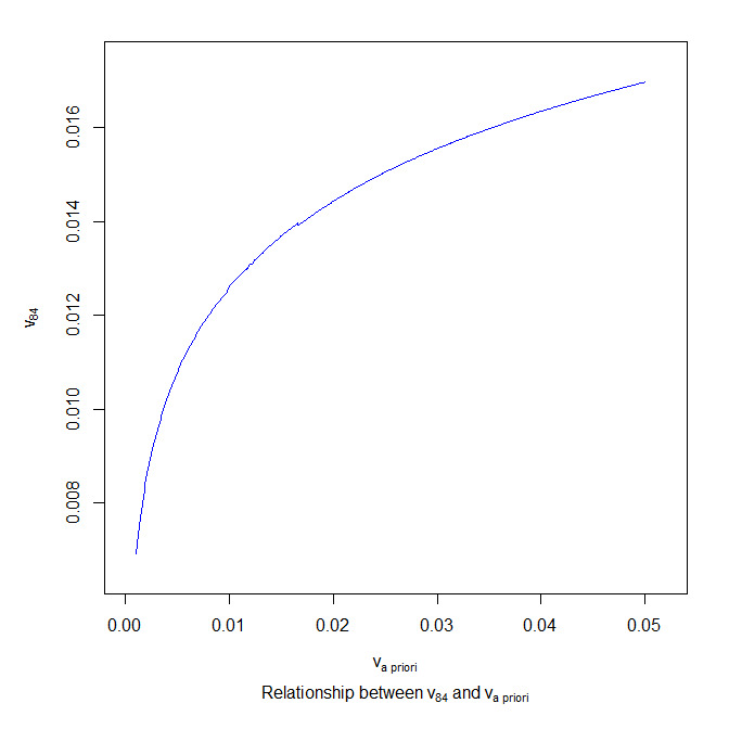
The emergence pattern at 84 months is particularly sensitive to the more leveraged a priori pattern relative to the empirically implied value. In this example, the a priori assumption of 0.04, compared with an implied empirical value of approximately 0.0136, pulls the Pattern Shrinkage estimate upward to approximately 0.0164, about 21% higher. We can transform the last column equation into a function of \(v_{84}\) and \(v_{a\ priori}\). The responsiveness to the a priori assumption in the last column equation can be visualized through the function in Figure 6.1:

\[\mathcal{F\ (}v_{a\ priori},\ v_{84})\ = \ 20\ - \ 1,497v_{84}\ - \ 5log(\frac{v_{84}}{v_{a\ priori}}).\]

It is easy to discern from Figure 6.1 that \(v_{84}\) is a concave-down function of \(v_{a\ priori}\) and increases at a diminishing rate. \(v_{84}\) can be quite sensitive to small changes in \(v_{a\ priori}\) at lower values.

Recall that \(v_{84}\) represents the emergence pattern in the last development period, where observed data are sparse and thus less credible. This strong responsiveness of later development periods to the a priori assumptions is actuarially sound and intuitive, as less credibility is assigned to the actual data compared to development periods with relatively more data, such as 12 or 24 months.

While the Pattern Shrinkage estimates from 36 to 84 months are all directionally pulled toward the a priori assumptions, the unity constraint prevents each development period from independently moving toward its respective a priori value. Increasing some \(v_{j}\)s necessarily forces compensating downward adjustments in others. The degree of responsiveness therefore reflects how the penalized row and column equilibrium allocates the influence of the penalty term across development periods. Earlier development periods such as 12 and 24 months, supported by substantially more observed data, remain more heavily anchored by the empirically implied patterns and therefore exhibit less responsiveness to the a priori assumptions.

From the second row equation, it is straightforward to obtain

\[v_{84} = 1\ - \ \frac{231}{u_{2020}}.\]

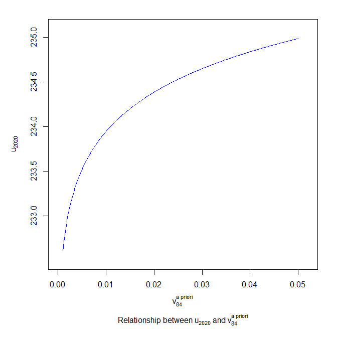
This function allows us to more directly visualize the interaction between the a priori emergence pattern and the estimated ultimate loss for AY2020 through Figure 6.2. Substituting this relationship back into the function of \(v_{84}\) and \(v_{a\ priori}\) and plotting the function between AY2020 and \(v_{a\ priori}\) over the range of interest, we have

\[\mathcal{F}\left( v_{a\ priori},\ u_{2020} \right) = \ 20\ - \ 1,497(1\ - \ \frac{231}{u_{2020}})\ - \ 5log(\frac{1\ - \ \frac{231}{u_{2020}}}{v_{a\ priori}}).\]

Via Pattern Shrinkage, not only are we able to formulate the estimated pattern as a function of the a priori pattern, we are also able to construct a linkage between accident-year ultimate loss and a priori pattern indirectly through the estimated pattern, thanks to the row and column equations under the penalized GLM framework. Figure 6.2 highlights the interdependency among a priori information, emergence patterns, and ultimate loss estimates. Small fluctuations in \(v_{a\ priori}\) at lower values can trigger relatively large changes in the estimate of \(u_{2020},\) as the AY2020 ultimate loss estimate is heavily influenced by the loss development in the last development period, age 84 months, where observed data are sparse and less credible. As a result, the penalty term exerts a stronger influence on the row and column equilibrium in later development periods, and this influence propagates recursively into the estimated ultimate losses through the row equations.

It is now apparent that Pattern Shrinkage embeds all three quantities—estimated development patterns, a priori patterns, and ultimate loss estimates—within a unified likelihood equilibrium. Consequently, changes in the a priori emergence assumptions directly alter the estimated ultimate losses as well as estimated emergence patterns through the jointly determined row and column equations equilibrium.

More importantly, these functional relationships closely mirror long-standing actuarial reserving practices. In real-world reserving applications, the last few development periods are often characterized by sparse, volatile, and low-credibility data. As a result, actuaries commonly supplement the observed experience with external benchmarks, industry studies, or judgmentally selected a priori assumptions. The responsiveness observed in the above two functions, \(\mathcal{F\ (}v_{a\ priori},\ v_{84})\) and \(\mathcal{F}\left( v_{a\ priori},\ u_{2020} \right)\), is therefore not merely a mathematical artifact of the penalized GLM framework, but rather a beautiful statistical reflection of how credibility naturally shifts toward external information when empirical data become thin.

In this sense, the penalized GLM framework provides a formal statistical interpretation of practical actuarial judgment. The framework quantitatively demonstrates how external benchmark assumptions propagate through the row and column equilibrium and influence both emergence patterns and ultimate loss estimates. Consequently, the methodology developed in this paper not only aligns with established actuarial intuition but also embeds this intuition directly within a unified likelihood-based estimation framework.

What if we are given a priori loss estimates? Suppose the a priori loss estimates in Table 6.5 are selected; further, assume λ = 5,000 (this value is selected for illustration purposes, to demonstrate a relatively strong degree of shrinkage toward the a priori loss estimate).

Similar to the process following Pattern Shrinkage, we can set up the following seven row equations under Ultimate Shrinkage based on equation (22):

\[\small \left( \begin{array}{r} 1,497\ - \ u_{2019}(v_{12} + v_{24} + v_{36} + v_{48} + v_{60} + v_{72} + v_{84})\ = \ 5,000\log(\frac{u_{2019}}{1,497}) \\ 231\ - \ u_{2020}(v_{12} + v_{24} + v_{36} + v_{48} + v_{60} + v_{72})\ = \ 5,000\log(\frac{u_{2020}}{530}) \\ 2,608\ - \ u_{2021}(v_{12} + v_{24} + v_{36} + v_{48} + v_{60})\ = 5,000\log(\frac{u_{2021}}{3,200}) \\ 585\ - \ u_{2022}(v_{12} + v_{24} + v_{36} + v_{48})\ = \ 5,000\log(\frac{u_{2022}}{595}) \\ 1,285\ - \ u_{2023}(v_{12} + v_{24} + v_{36})\ = 5,000\log(\frac{u_{2023}}{1,978}) \\ 1,324\ - \ u_{2024}(v_{12} + v_{24})\ = \ 5,000\log(\frac{u_{2024}}{2,498}) \\ 428\ - \ u_{2025}v_{12}\ = \ 5,000\log(\frac{u_{2025}}{1,603}) \end{array} \right.\ \]

We can set up the column equations based on equation (23) along with the unity constraint:

\[\left\{ \begin{array}{r} v_{12} + v_{24} + v_{36} + v_{48} + v_{60} + v_{72} + v_{84} = 1 \\ v_{12} = \frac{4,056}{u_{2019} + u_{2020} + u_{2021} + u_{2022} + u_{2023} + u_{2024} + u_{2025}} \\ v_{24} = \frac{1,866}{u_{2019} + u_{2020} + u_{2021} + u_{2022} + u_{2023} + u_{2024}} \\ v_{36} = \frac{1,017}{u_{2019} + u_{2020} + u_{2021} + u_{2022} + u_{2023}} \\ v_{48} = \frac{643}{u_{2019} + u_{2020} + u_{2021} + u_{2022}} \\ v_{60} = \frac{298}{u_{2019} + u_{2020} + u_{2021}} \\ v_{72} = \frac{58}{u_{2019} + u_{2020}} \\ v_{84} = \frac{20}{u_{2019}} \end{array} \right.\ \]

With the structurally reducible nature of these two systems of equations in mind, similar to the approach for Pattern Shrinkage, we can now solve these equations recursively by first solving for \(u_{2019}\) in the first row equation, then \(v_{84}\) in the last column equation—rinse and repeat.

Before turning to the results, let us examine the functions to predict what the results will look like. The first row equation, which ultimately predicts the loss estimate for AY2019 (the most mature year), while statistically sound, is actuarially meaningless since no tail development is assumed and thus the AY2019 ultimate loss would just be the cumulative loss to date, which is 1,497. It is then very easy to obtain \(u_{2019}\ = \ 1,497\) and \(v_{84} = 0.014.\) This is one important instance in which actuarial judgment and practical industry considerations appropriately supersede purely statistical estimation.

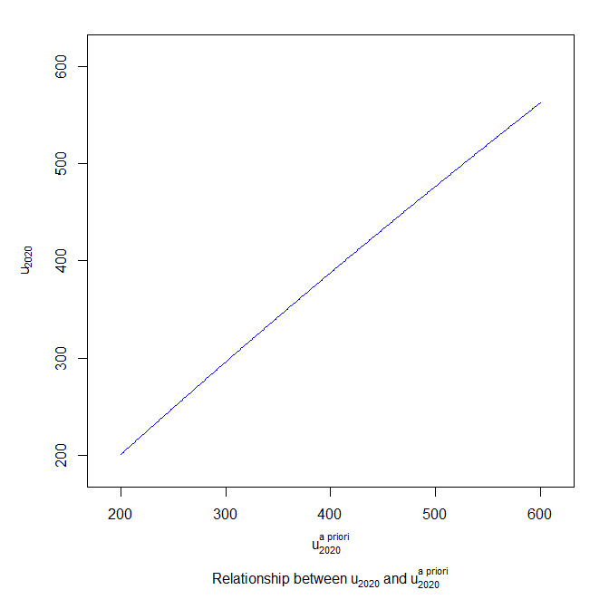
The second row equation, which solves for the ultimate loss estimate for AY2020, can then be simplified into the functional form

\[\mathcal{F}\left( u_{2020}^{a\ priori},\ u_{2020} \right) = 231\ - \ 0.986u_{2020}\ - \ 5,000\ log(\frac{u_{2020}}{u_{2020}^{a\ priori}}).\]

From Figure 6.3, we can see that \(u_{2020}\) monotonically increases as the a priori loss estimate increases. This monotonic increase and seeming overreliance on the a priori loss estimate for AY2020 closely mirror actuarial practices. We need to predict the loss development for AY2020 only in month 84, and that period is the latest development period, where observed data are sparse and volatile and where, in practice, actuaries often rely more heavily on industry benchmarks or other external a priori estimates. This function formally quantifies this real-world behavior. This behavior is strikingly similar to how the estimated emergence pattern is getting pulled directionally toward the a priori pattern in the most recent development period, as shown earlier.

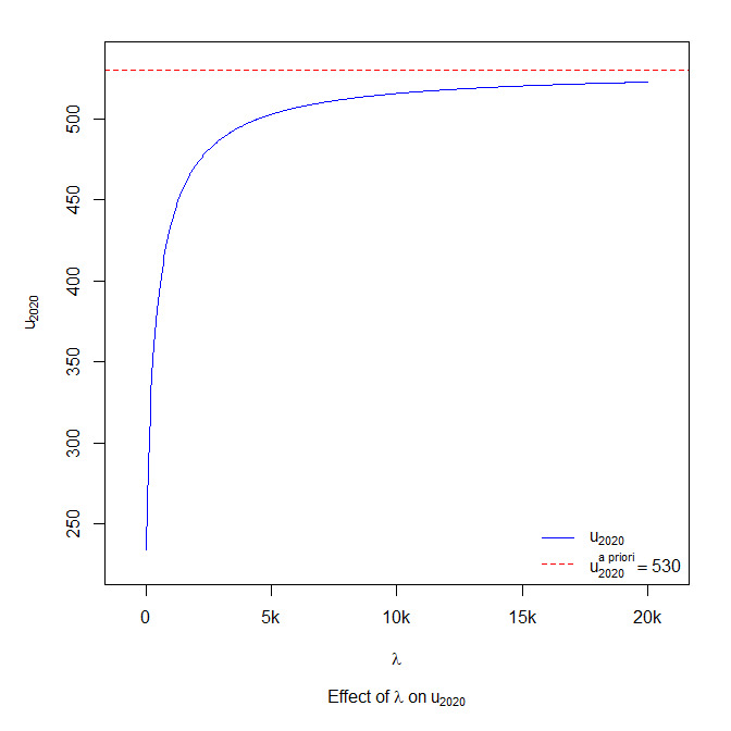
An interesting question regarding the sensitivity of the penalty parameter in Ultimate Shrinkage was raised during the review of this paper. Assuming the a priori loss estimate of 530 for AY2020 is fixed, to isolate the effect of the penalty parameter, we consider the following simplified estimating function relating the AY2020 ultimate loss estimate to its selected penalty parameter:

\[\mathcal{F}\left( \lambda,\ u_{2020} \right) = 231\ - \ 0.986u_{2020}\ - \ \lambda\ log(\frac{u_{2020}}{530}).\]

Figure 6.4 reinforces the idea that the ridge penalty term is essentially a credibility-weighting mechanism that pulls the ultimate loss estimate toward the a priori loss estimate as the penalty parameter approaches infinity.

The penalized estimates for various values of \(\lambda\) are shown in Table 6.6:

For small values of \(\lambda\) (e.g., 5 and 50), the penalized estimate remains close to the unpenalized GLM estimate, indicating that the observed data dominate the estimation and that the pulling force of credibility weighting is weak. As \(\lambda\) increases to 500 and 5,000, progressively greater weight is assigned to the a priori estimate, producing substantial shrinkage while still maintaining the continuity of the solution. For very large values of \(\lambda\), the estimates change only marginally because the solution converges asymptotically to the a priori value rather than crossing it.

These results confirm that the penalty parameter operates in the intended manner. Rather than producing an abrupt switch between the unpenalized estimate and the selected prior, increasing the penalty parameter results in a gradual and predictable increase in the influence of the a priori estimate. This behavior is consistent with the theoretical objective of ridge regularization and supports interpreting the penalty parameter as a credibility-type weighting mechanism that balances empirical experience with actuarial judgment.

Table 6.7 outlines the Ultimate Shrinkage estimates as compared with the estimates from the unpenalized GLM.

The results demonstrate that the ridge penalty does not apply a uniform degree of shrinkage across accident years. Instead, the magnitude of shrinkage depends on the discrepancy between the unpenalized GLM estimate and the selected a priori estimate as well as the structural position of each accident year within the recursive row and column equation equilibrium.

For AY2020, the unpenalized GLM estimate is noticeably lower than the selected a priori estimate (234 versus 530). Under the chosen penalty parameter, the penalized estimate increases to 503, reducing the gap between the unpenalized GLM estimate and the selected a priori estimate and moving approximately 91% of the way from the unpenalized estimate toward the a priori estimate, which highlights the strong influence of the selected prior when empirical information at age 84 months is limited. By contrast, the remaining accident years exhibit smaller changes, generally between approximately 10% and 43%, while AY2022 decreases by 9% because the selected a priori estimate is lower than the unpenalized estimate. These results demonstrate that the direction of shrinkage is determined by the relationship between the empirical estimate and the selected prior, with the penalty moving the estimate toward the prior regardless of whether an increase or decrease is required. Collectively, these results establish the ridge-penalized GLM as an effective credibility-based mechanism for integrating empirical loss experience and a priori information in ultimate loss estimation.

7. Conclusion

This paper represents an initial exploration of stochastic loss reserving using penalized GLMs. Through the lens of likelihood functions, the paper has shown that a penalized GLM framework can be implemented as a credibility-weighted reserving technique incorporating either a priori development patterns or a priori expected loss estimates, providing much more flexibility and autonomy than a deterministic BF method. The equilibrium between the row and column equations presented in the penalized GLM framework reflects the credibility-weighting nature of the penalized GLM reserving method and introduces simultaneous dependency among a priori information, development patterns, and ultimate loss estimates that is absent in other traditional deterministic reserving methods.

Beyond this initial exploration, further topics of research interest that could be of tremendous value in this domain include the following:

• Quantification of responsiveness and sensitivity due to the a priori information in the penalized GLM framework

• Selection of an optimal penalty parameter in the penalized GLM framework for stochastic loss reserving, and detailed analyses and quantification of sensitivity of estimations due to the penalty parameter