Attribution of Loss Development Dynamics: A Bayesian Structural Time Series Approach

1. Introduction

Accurate estimation of loss reserves remains one of the central challenges in property and casualty actuarial practice. At its core, reserving requires projecting future claim development from historical experience, often under conditions of uncertainty, structural change, and incomplete information. A recurring difficulty is distinguishing the underlying drivers of observed loss patterns. Changes in reported losses may reflect trends, operational or legal changes, calendar-year (CY) effects, or isolated shocks. In practice, such influences are often intertwined, making it difficult to isolate their contributions and assess persistence.

This challenge has long been recognized in actuarial literature. For example, Barnett and Zehnwirth (2000) emphasized the importance of understanding the structure of loss data rather than relying solely on mechanical application of traditional methods. Their work highlights a fundamental tension in reserving: Whereas historical data provide the primary basis for estimation, such data do not always reflect a stable or homogeneous process.

In practice, actuaries routinely confront questions such as: Is an observed increase in losses indicative of a sustained trend or a temporary fluctuation? Does a sudden change reflect a structural shift—such as a change in claims handling or legal environment—or simply noise? Are CY effects masking underlying accident-year development patterns? Such questions influence trend assumptions, development factors, ultimate loss estimates, and explanatory variables in reserving models. Misattribution can lead to biased projections, either by overreacting to short-term volatility or by failing to recognize genuine structural change.

Traditional reserving frameworks do not explicitly separate these effects. Methods such as chain ladder (i.e., loss development method) and Bornhuetter–Ferguson implicitly combine multiple sources of variation into aggregate development patterns. While effective, they offer limited transparency into observed changes. As a result, actuaries often rely on supplemental diagnostics, such as CY analyses, residual plots, or ad hoc adjustments—which may lack a systematic structure and depend heavily on judgment.

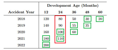
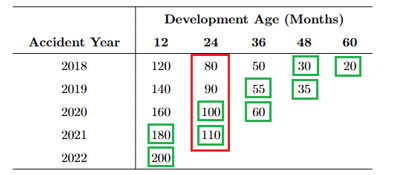
One way to address this limitation is to view reserving data through the lens of time series analysis. A loss development triangle can be interpreted not only as a two-dimensional structure indexed by accident year and development age but also as a collection of one-dimensional time series. Fixing a development age yields an AY series of incremental losses across origin periods, while summing along diagonals produces a CY series reflecting loss emergence over time. These perspectives provide complementary views of the same underlying process.

Within each series, observed values can be interpreted as arising from a combination of components, such as baseline level, trend, seasonal effects, structural breaks (i.e., abrupt changes in the underlying process, such as shifts associated with inflation shocks, claims handling changes, or tort reform), and random noise. These components are treated as latent drivers inferred from the observed time series. Decomposing the series into such elements provides a structured framework for interpreting observed changes and assessing their likely persistence. Section 2 and Appendix A discuss the components and their interpretation in greater detail. Readers unfamiliar with BSTS or state-space modeling concepts may find it helpful to review Appendix A before proceeding. The appendices for this paper may be accessed in the Data Sets/Files tab on this page.

Motivated by these considerations, this paper develops a Bayesian state-space framework for analyzing reserving data as time series and decomposing observed loss patterns into interpretable components. The objective is not to replace traditional reserving methods, but to complement them by providing additional insight into the structure of the data and the nature of observed changes. In doing so, the paper addresses a central question in actuarial practice: not only how losses are developing, but why they are developing in that manner.

2. Bayesian structural time series

The perspective developed above—viewing reserving data as a collection of time series and seeking to interpret their underlying structure—naturally leads to the question of how such decomposition can be carried out in a systematic and coherent way. Bayesian structural time series (BSTS) models provide a flexible framework for this purpose (Harvey 1989; Scott and Varian 2014).

BSTS treats the observed series as the manifestation of latent components—such as level, trend, seasonality, and structural effects—that evolve over time. Those components are inferred from the data, allowing the model to represent complex dynamics in a structured, interpretable manner.

A defining feature of BSTS is its Bayesian formulation. Both the latent states and model parameters are treated as random variables with prior distributions, and inference is based on the posterior distribution:

$$p\left( \theta,\alpha_{1:T}\mid y_{1:T} \right) \propto p\left( y_{1:T}\mid\alpha_{1:T},\theta \right)\text{ }p\left( \alpha_{1:T}\mid\theta \right)\text{ }p(\theta),$$

where $\theta$ denotes model parameters and $\alpha_{1:T}$ represents the latent state vectors. This framework explicitly incorporates uncertainty into both the estimated components and forecasts.

Within this structure, different sources of variation can be represented through separate components, while prior distributions constrain their behavior based on reasonable assumptions about how loss development evolves. This is important in reserving applications, where time series are often short and noisy, and unconstrained decomposition may lead to unstable or non-interpretable results.

The flexibility of the framework also allows for the inclusion of structural interventions, such as level shifts or regime changes, which can be incorporated through regression-style components with appropriate prior specification. In this way, BSTS provides a unified approach for representing both gradual evolution and discrete structural change within a single probabilistic model.

While Bayesian methods have been applied in actuarial contexts, their use in decomposing reserving-related time series remains limited. Traditional approaches focus on development patterns within the loss triangle and do not explicitly model the underlying structural drivers in a unified framework.

In this paper, BSTS is applied to time series derived from loss development data with the goal of analyzing how structural effects are represented and attributed within the model. All BSTS models in this study were implemented in R using the bsts package (Scott 2025), which performs Bayesian estimation internally using Markov Chain Monte Carlo (MCMC) methods. The specific model components, prior choices, estimation details, and supporting time series concepts used in this study are described in the “BSTS Model Specification” section below and Appendix A.

3. Methodology and experimental design

3.1. Data construction and time series definitions

The analysis represents loss development triangles as collections of one-dimensional time series. From incremental loss data indexed by accident period and development age, two series types are constructed:

• Accident-year (AY) series: For a fixed development age, incremental losses are tracked across accident periods.

• Calendar-year (CY) series: Incremental losses are aggregated along diagonals of the triangle.

These provide complementary perspectives: AY series isolate development-age behavior, while CY series reflect aggregate loss emergence over time, as illustrated in Figure 1. Only fully observed CY diagonals are retained, and minimum length requirements are imposed to ensure reliable estimation. Extensions incorporating partially observed diagonals, hierarchical borrowing across related series, or multivariate state-space structures may help relax these constraints and represent a potential area for future research.

Figure 1.Time series generation—CY series is equivalent to the series of sums along each diagonal (green boxes), while AY series for a given maturity is generated by summing a single column (red box).

3.2. Data sources and characteristics

The experiments in this study rely on two distinct data settings: simulated data generated from a controlled data-generating process (DGP) and real-world insurance reserving data.

Simulated data (Experiment 1)

Synthetic data are generated to reflect key reserving features, including stochastic level and trend, quarterly seasonality, structural breaks, and development-age effects. Observations are drawn from a gamma distribution to reflect positive, right-skewed loss behavior. Because the true components are known, this setting enables direct evaluation of component recovery.

Real data (Experiments 2, 3, and 4)

Real-world loss triangles of incurred losses and allocated loss adjustment expenses (LAE) are used

• Experiment 2—Workers’ compensation: Long-tailed data used to evaluate forecasting performance over extended development horizons.

• Experiments 3 and 4—Private passenger auto bodily injury liability: Shorter-tailed, more volatile data used to evaluate attribution under more dynamic conditions.

Datasets are anonymized and slightly modified while preserving structural characteristics.

3.3. BSTS model specification

All BSTS models in this study are formulated within a state-space framework with additive components. For a given time series $y_{t}$, the model is specified as

$$y_{t} = \mu_{t} + \delta_{t} + \gamma_{t} + x_{t}^{\prime}\beta + \varepsilon_{t},$$

where

• $\mu_{t}$: local level

• $\delta_{t}$: stochastic trend

• $\gamma_{t}$: seasonal component (quarterly where applicable)

• $x_{t}$: regression covariates representing structural breaks

• $\varepsilon_{t} \sim N(0,\sigma^{2})$: observation noise

The latent states evolve according to a local linear trend specification:

$$\mu_{t} = \mu_{t - 1} + \delta_{t - 1} + \eta_{t},$$

$$\delta_{t} = \delta_{t - 1} + \zeta_{t},$$

where $\delta_{t}$ represents the slope (trend) and disturbances ($\eta,\ \zeta$) are assumed Gaussian.

Structural breaks are modeled using step-function indicators. In simulated data, break locations are fixed; in real data, candidate breakpoints are estimated using spike-and-slab priors (Scott and Varian 2014; see Appendix A), enabling automatic selection by shrinking weak breakpoint coefficients toward zero.

Models are estimated using MCMC with standard burn-in, and posterior summaries are based on sampled draws. While simulated data are generated under a gamma observation process, estimation assumes Gaussian noise.

3.4. Experimental design

Four experiments are conducted, each addressing a distinct aspect of model performance.

Experiment 1: Component recovery under known DGP

Simulated data with known latent components are used to evaluate the BSTS’s ability to recover

• level,

• trend,

• seasonality,

• structural breaks, and

• noise.

The data are generated from an additive structural process designed to reflect common features of reserving data. Specifically, a latent signal is constructed as the sum of a local linear trend component (stochastic level and slope), a seasonal component, and structural breaks implemented as step changes in the level. This latent signal defines the conditional mean of the observed series.

Observed values are then generated from a gamma distribution, with mean equal to the latent signal and variance governed by a fixed dispersion parameter. This introduces realistic features such as positivity and right-skewness, which are characteristic of insurance loss data.

This formulation yields a controlled environment in which the true underlying components are known by construction, while also introducing a degree of model misspecification, as BSTS is estimated under a Gaussian observation assumption. As a result, the experiment provides insight not only into component recovery under ideal conditions, but also into the robustness of BSTS when applied to data with distributional properties consistent with real-world reserving contexts.

Experiment 2: Forecasting performance comparison

Experiment 2 evaluates the out-of-sample forecasting performance of BSTS models relative to commonly used benchmark methods. For each constructed time series (accident-year and calendar-year), a rolling holdout framework is applied in which the final three observations are reserved for out-of-sample evaluation.

Forecasts are generated using multiple modeling approaches, including standard benchmark forecasting methods commonly used in time series analysis (Hyndman and Athanasopoulos 2021)

• BSTS specifications with varying component structures (e.g., level with breaks, level with breaks and AR(1) serial correlation term, trend with breaks)

• Ordinary least squares (OLS) trend models

• Drift and naïve benchmark methods

To improve model stability and align with the multiplicative nature of loss development, incremental losses are transformed prior to model fitting using a logarithmic transformation of the form

$$y_{t} = \log\left( incremental\ loss_{t} + 1 \right).$$

This transformation is applied consistently across all forecasting methods. By operating on the log scale, multiplicative growth patterns are converted into an additive structure, making them more amenable to linear and state-space modeling. In addition, the transformation reduces the influence of extreme observations and large fluctuations in incremental losses, thereby improving parameter stability and forecast robustness.

All models are estimated on the transformed scale, and forecasts are generated accordingly. Predicted values are then transformed back to the original scale for evaluation, ensuring that forecast accuracy metrics—such as mean absolute error (MAE), mean squared error (MSE), and mean absolute percentage error (MAPE)—are interpretable in monetary terms.

Forecast performance is assessed over the holdout period using these standard error metrics, allowing for a direct comparison of predictive accuracy across modeling approaches.

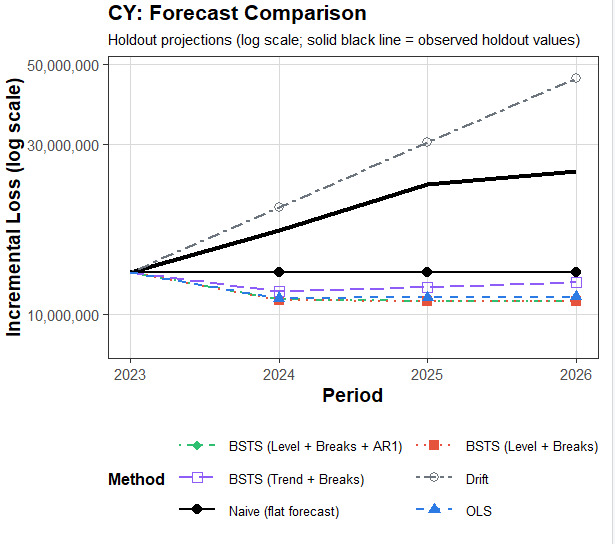
For visualization purposes, forecast comparison plots are displayed on a logarithmic (base 10) scale. This visual scaling facilitates comparison across series with differing magnitudes and highlights relative differences in forecast trajectories but is distinct from the natural logarithm transformation used in model estimation.

Experiment 3: Perturbation and attribution analysis

Experiment 3 evaluates the interpretability of BSTS decompositions by examining how controlled structural perturbations are represented within the model. Rather than assessing attribution in terms of strict recovery accuracy, this experiment is designed to study how structural signals are expressed and distributed across components within the BSTS framework, particularly in the presence of transformations between CY and AY views of the data.

The procedure is as follows:

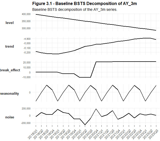
1. Fit a baseline BSTS model to each time series (the “ground-truth” decomposition).

2. Extract the estimated components (level, trend, seasonality, break effect, and noise).

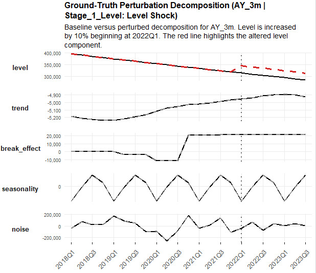
3. Introduce perturbations to one component at a time, while holding all other components fixed.

4. Reconstruct a synthetic observed series by recombining the perturbed components.

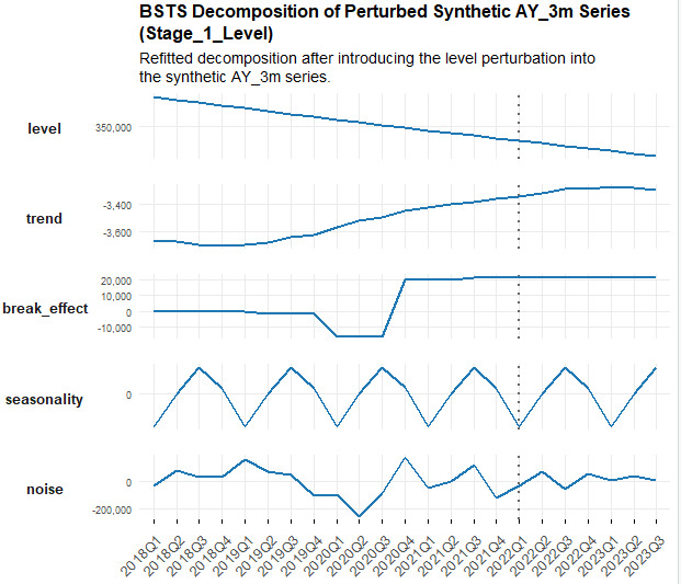
5. Refit the BSTS model to the perturbed series to assess whether the induced change is correctly recovered and attributed to the perturbed component.

6. Compare the resulting decomposition to the known perturbation, focusing on how the induced signal is distributed across components.

The objective of this experiment is not to determine whether BSTS “correctly” recovers the perturbed component in a one-to-one sense. Instead, the analysis examines how a structural change introduced in one component is reexpressed within the decomposition, providing insight into how different types of signals manifest under the BSTS representation.

Because the true underlying components are not observable in real data, the baseline decomposition is treated as a reference structure. Perturbations are applied directly to this structure, allowing for a controlled comparison between the known induced change and the model-implied attribution following refitting.

Perturbations are applied to the following components

1. Level (step shifts)

   Sudden, persistent changes in the baseline level of losses are introduced at a specified point in time.

   Example: A permanent increase in claim severity due to a change in policy limits, benefit structures, or underwriting mix (e.g., a shift toward higher-risk insureds).

2. Trend (slope changes/ramps)

   Changes in the rate of growth or decline are introduced, typically in the form of a gradual increase or decrease in slope over time.

   Example: A sustained increase in loss costs driven by inflation (e.g., medical cost inflation in workers’ compensation or Consumer Price Index (CPI)–driven severity increases in auto liability).

3. Seasonality (pattern distortions)

   The magnitude or structure of recurring seasonal patterns is modified, either by amplifying or dampening periodic effects.

   Example: Changes in claim reporting or occurrence patterns due to weather cycles, legislative reporting deadlines, or operational shifts that alter quarterly claim emergence behavior.

4. Noise (volatility bursts)

   Temporary increases in variability are introduced without altering the underlying structural signal.

   Example: Random fluctuations arising from large losses, reserve strengthening on individual claims, or short-term operational disruptions that increase volatility without changing long-term expectations.

Note that although level shifts and structural break effects can produce similar observed patterns, level perturbations represent endogenous baseline changes (e.g., sudden shift in underwriting mix toward higher-risk insureds, a change in policy limits, etc.), while break effects represent discrete exogenous intervention events (e.g., tort reform, legislative changes, external inflation shocks, etc.). Structural break components are not explicitly perturbed, as they already represent discrete interventions in the underlying process. Further perturbation of these effects would effectively constitute a “perturbation of a perturbation,” making interpretation less meaningful in a reserving context.

This experimental design enables a controlled examination of how different types of structural changes are represented within BSTS decompositions. In particular, it highlights the extent to which a perturbation introduced in one component may be distributed across multiple components upon refitting. This behavior is especially relevant when comparing CY and AY representations, as the transformation between these perspectives can alter the temporal signature of a signal, leading to different but still coherent representations within the model.

Overall, Experiment 3 provides a diagnostic framework for understanding how BSTS interprets structural changes in reserving data. The results offer insight into the mapping between underlying drivers and their representation in decomposed components, emphasizing that component-level attribution should be interpreted as a structured representation of the signal rather than a direct identification of its original source.

Experiment 4: Calendar-year perturbations in accident-year space

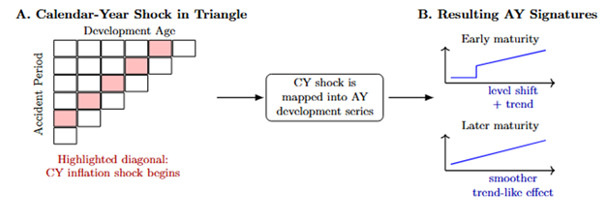
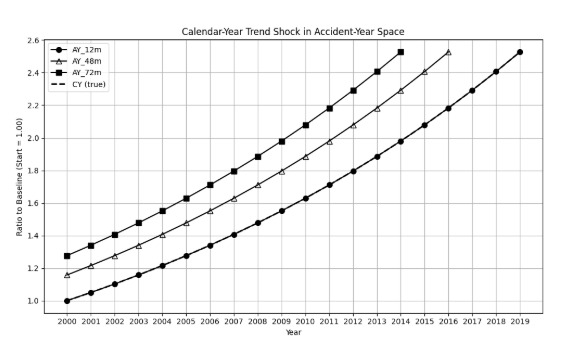
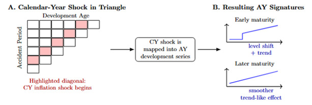
This experiment examines how perturbations defined in CY space manifest when observed through AY development series (see Figure 2). In contrast to prior experiments, where perturbations are applied directly to the modeled time series, this setup introduces shocks in a coordinate system that differs from the one used for decomposition. As a result, the experiment is designed to evaluate how structural effects defined in CY space are represented within AY-based BSTS decompositions.

Let $y_{c}^{CY}$denote incremental losses in calendar year $c$, and $y_{t,d}^{AY}$denote incremental losses for accident year $t$ at development age $d$. The relationship between the two representations is given by

$$c = t + d,$$

so that each observation in an AY development series corresponds to a specific calendar year.

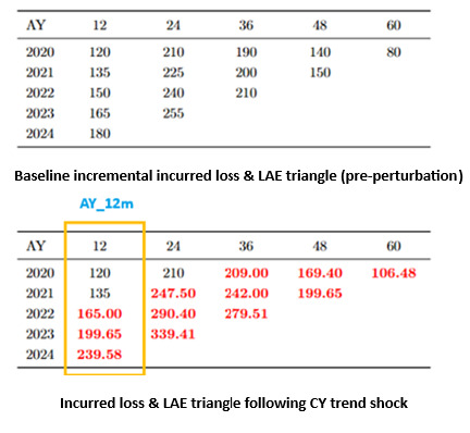
A baseline incremental triangle is first constructed to exhibit a realistic long-tail development pattern. This baseline serves as the unperturbed reference against which all subsequent transformations are measured.

For the experiments presented below, CY perturbations are introduced at fixed calendar-year periods chosen to provide sufficient pre- and post-intervention observations for analysis. Specifically, the level perturbation begins in 2022Q1, the trend and noise perturbations begin in 2021Q3, and the seasonal perturbation begins in 2020Q1.

Figure 2.Illustration of CY shocks across AY maturities. A CY shock affects diagonal cells in the triangle but may appear as different combinations of level, trend, and break behavior when viewed through individual AY development series.

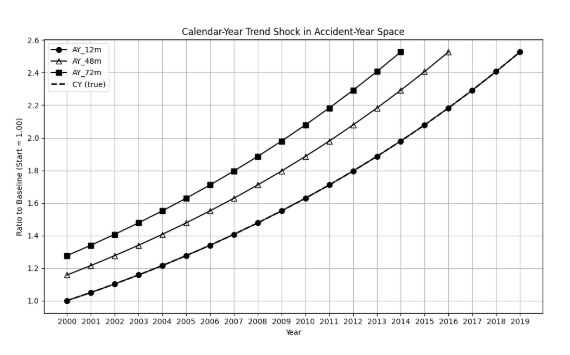
(1) Trend (inflation) shock

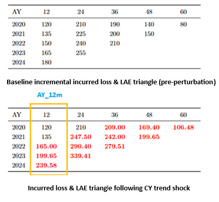
To illustrate the CY-to-AY mapping, suppose a calendar-year trend shock begins at calendar year $c_{0}$. Let $X_{c}$ denote the baseline incremental loss in CY $c$, and define the shocked series as

$$X_{c}^{*} = X_{c}\text{ }g(c),$$

where

$$g(c) = \left\{ \begin{matrix} 1, & c < c_{0}, \\ \left( 1+i)^{\text{ }c - c_{0}} \right., & c \geq c_{0}, \end{matrix} \right.\ $$ and $i$ is the inflation rate.

Using the identity $c = t + d$, the corresponding AY representation is

$$X_{t,d}^{*} = X_{t,d}\text{ }g(t + d).$$

Fix an accident period $t$ and consider its development over $d$. The shock first appears when $t + d = c_{0}$, i.e., at development period

$$d_{0} = c_{0} - t.$$

For $d < d_{0}$, the series is unaffected. At $d = d_{0}$, the inflation process begins, but the first affected observation remains at the baseline level. For $d > d_{0}$, the factor evolves as

$$g(t + d) = (1 + i)^{d - d_{0}},$$

which increases smoothly with development.

Thus, as Figure 3 shows, within a single AY series, the effect of a CY trend shock takes the form of a transition point at the first affected development period d₀, followed by a systematic multiplicative upward annual trend factor of (1 + i).

This pattern is most clearly observed at earlier maturities, where the transition from unaffected to affected periods occurs within the observed development window.

Motivation. In practice, CY-driven effects such as medical cost inflation, litigation trends, and changes in claim severity often emerge gradually over time rather than as discrete shifts. The result above shows that when such effects are viewed in an AY framework, they may not appear as a pure trend within any single series. Instead, the impact may present as an initial shift followed by continued growth, with the timing and shape depending on maturity. As a result, when applying BSTS, these real-world drivers may be reflected not as a single component but as a combination of level changes, trend, and potentially other structural elements. This highlights the importance of interpreting model outputs in the context of how CY effects propagate through the data.

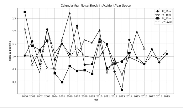
(2) Noise (variance) shock

A variance shock is introduced in CY space by increasing the dispersion of incremental values beginning at CY $c_{0}$. Let $X_{c}$ denote the baseline CY incremental loss, and define the shocked series as

$$X_{c}^{*} = X_{c}\text{ }(1 + \varepsilon_{c}),c \geq c_{0},$$

where $\varepsilon_{c}$is a mean-zero random disturbance with elevated variance. For $c < c_{0}$, the series remains unchanged.

Using the identity $c = t + d$, the corresponding AY representation is

$$X_{t,d}^{*} = X_{t,d}\text{ }(1 + \varepsilon_{t + d}).$$

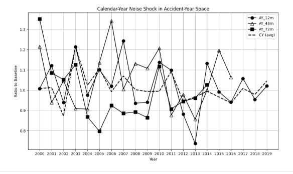
Thus, each AY cell inherits the noise associated with the CY diagonal to which it belongs. Because $\varepsilon_{t + d}$ is random and does not evolve systematically with accident period or development period, the induced effect in AY space remains noise-like rather than trend-like or level-shift-like.

Motivation. This perturbation is intended to reflect real-world periods of heightened volatility or uncertainty in claim emergence, such as operational disruptions, reporting delays, changes in claims handling practices, or external shocks. When such volatility is calendar-year driven, it affects all open claims in the affected period. In an AY view, this should still appear primarily as irregular fluctuation rather than as a persistent shift in level or trend, although some apparent structure may emerge at particular maturities due to the CY-to-AY transformation.

Transformation to AY development series

For each perturbation type, the resulting CY-adjusted values are reassembled into an AY incremental triangle. This transformation allows the same underlying CY perturbation to be viewed through multiple development-age perspectives. Rather than combining the resulting AY decompositions into a single attribution measure, the collection of AY series is examined to evaluate how the CY perturbation manifests across development maturities. From this triangle, individual AY development series (e.g., $AY_{12m},\ AY_{24m},\ldots$) are extracted and analyzed independently using BSTS decomposition. Consistency of attribution patterns across maturities is interpreted as evidence of a coherent underlying CY signal, while differences across maturities help characterize how the CY-to-AY transformation alters the apparent structure of that signal.

To facilitate comparison across maturities and perturbation types, all series are expressed on a ratio-to-baseline basis, where each observation is scaled relative to its corresponding value in the unperturbed triangle.

Figure 3.Incremental incurred loss and LAE triangle with a 10% CY trend shock beginning in CY 2022. Shocked cells are shown in bold red.

3.5. Evaluation metrics

Model performance is evaluated using metrics tailored to the specific objective of each experiment. For Experiments 1 and 2, standard accuracy measures are retained to assess component recovery and forecast performance, respectively. For Experiments 3 and 4, however, the evaluation framework is redesigned to directly measure attribution accuracy under controlled perturbations.

Experiments 1 and 2

For component recovery (Experiment 1) and forecasting accuracy (Experiment 2), standard error metrics are used:

• Mean absolute error (MAE):

$$\text{MAE} = \frac{1}{n}\sum \mid y_{t} - {\widehat{y}}_{t} \mid .$$

• Root mean squared error (RMSE):

$$\text{RMSE} = \sqrt{\frac{1}{n}\sum(y_{t} - {\widehat{y}}_{t})^{2}}.$$

• Mean absolute percentage error (MAPE):

$$\text{MAPE} = \frac{1}{n}\sum \mid \frac{y_{t} - {\widehat{y}}_{t}}{y_{t}} \mid \times 100.$$

These metrics provide familiar and interpretable summaries of overall accuracy. In cases where values approach zero (e.g., noise or seasonal components), stabilized versions of MAPE are used to ensure numerical robustness.

Experiments 3 and 4: Attribution-based metrics

Experiments 3 and 4 focus on how BSTS distributes a known structural perturbation across its decomposed components. The analysis uses a percentage-based allocation framework that directly quantifies how the model assigns the induced signal.

For each perturbation experiment, two quantities are constructed.

The true perturbation signal, defined as the difference between the perturbed and baseline component paths for the targeted component.

The estimated perturbation signal, defined as the difference between the refitted BSTS decomposition and the baseline BSTS decomposition from the unperturbed series, is evaluated across all components.

Let $\Delta_{j}^{\text{est}}(t)$ denote the estimated perturbation attributed to component $j$ after refitting.

To summarize attribution, the total magnitude of the estimated perturbation assigned to each component is computed as

$$A_{j} = \sum_{t}^{}{\mid \Delta_{j}^{\text{est}}(t) \mid}.$$

These quantities represent the total signal (in absolute terms) that the BSTS model assigns to each component.

The percentage allocation to component $j$ is then defined as

$$\text{Allocation}_{j} = \frac{A_{j}}{\sum_{l}^{}A_{l}} \times 100\%.$$

This produces a normalized distribution of the total estimated perturbation signal across all components $l$ (level, trend, seasonality, break effect, and noise).

Interpretation

Under this framework:

• The diagonal element (i.e., allocation to the perturbed component) represents the proportion of the signal that BSTS attributes to the “correct” component.

• The off-diagonal elements represent how the signal is redistributed across other components.

Importantly, this approach does not attempt to measure correctness in an absolute sense but rather characterizes how the model internally represents the perturbation.

This aligns directly with the objective of Experiment 3: to understand how structural signals are expressed within the BSTS decomposition, rather than whether they are recovered exactly.

3.6. Time series length, granularity, and prior specification

The time series used in this study are relatively short (approximately 16–23 observations), reflecting the data constraints typical of actuarial reserving practice. While shorter than those used in many statistical applications, this setting is representative of real-world reserving environments.

A key trade-off arises across development maturities. Earlier development periods provide longer histories but tend to exhibit greater volatility, while more mature development ages are generally more stable but supported by fewer observations due to triangle truncation. The use of accident-quarter (AQ) data increases temporal resolution and enables modeling of seasonal effects, partially mitigating these limitations.

However, short time series also create identifiability challenges, as different combinations of structural components (e.g., level, trend, and noise) may produce similar observed behavior. This is particularly relevant in reserving data, where gradual changes and structural shifts may overlap and be difficult to distinguish.

BSTS addresses such limitations through the use of prior distributions that regularize component behavior and stabilize estimation. In this study, priors were selected to reflect typical reserving dynamics—gradual evolution, persistence, and limited high-frequency volatility—while still allowing for meaningful structural changes. Structural break components are governed by spike-and-slab priors, which allow candidate breakpoints to be considered while shrinking weak effects toward zero. Together, these priors help reduce overfitting and improve interpretability in short and noisy reserving time series.

Overall, the data environment considered in this study reflects practical reserving conditions and provides a realistic setting for evaluating model behavior.

4. Results

4.1. Overview

This section presents the results of the four experiments described in Section 3.

4.2. Experiment 1: BSTS component recovery under known DGP

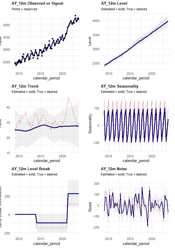
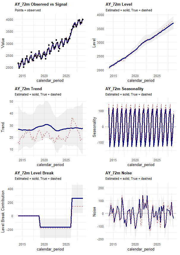
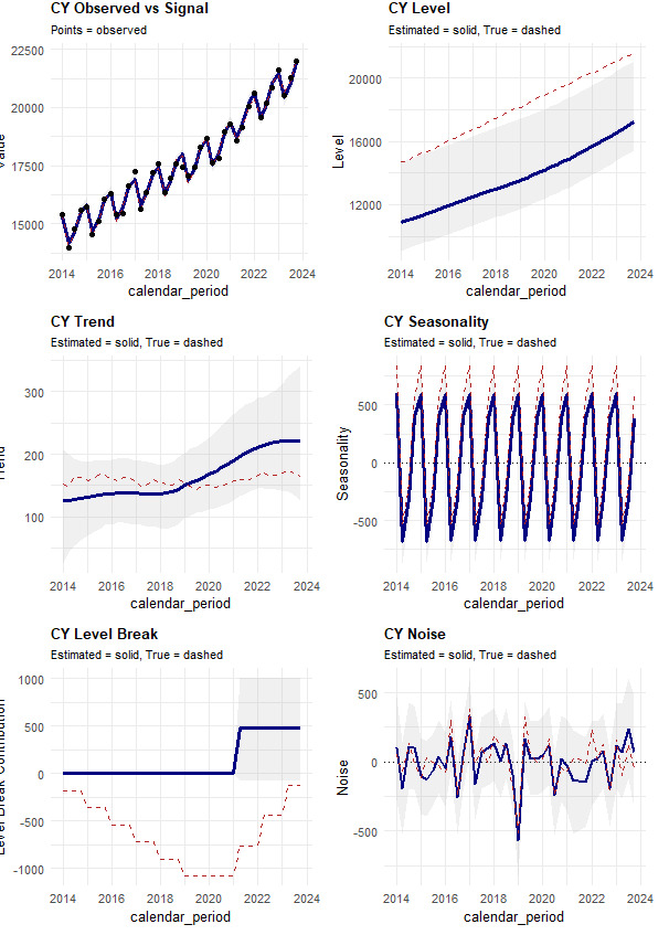
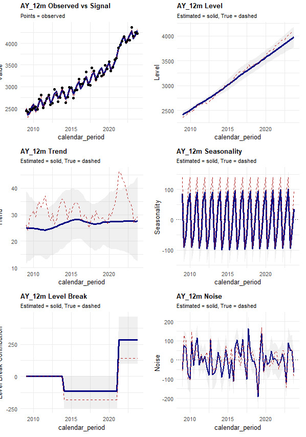
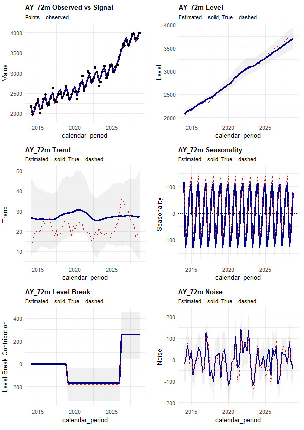
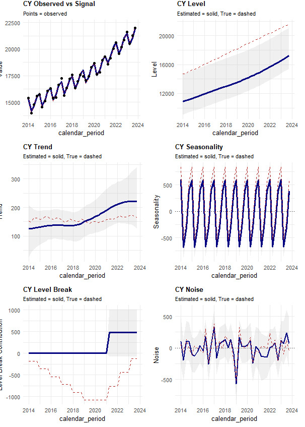
For illustrative purposes, results on the following pages are presented for the 12-month development accident-year series (AY_12m), the 72-month development accident-year series (AY_72m), and the calendar-year (CY) series, representing early development, mature development, and aggregated loss emergence, respectively. Here, AY_Xm denotes the time series of incremental losses at X months of development tracked across accident periods (e.g., AY_12m represents incremental losses at 12 months of development for successive accident periods). Complete results for all series—AY_12m, AY_24m, AY_36m, AY_48m, AY_60m, AY_72m, and CY—are provided in Appendix C.

Figures 4 through 6 present the BSTS decompositions for each of these series, showing the observed time series alongside the estimated latent components, including level, trend, seasonality, structural break effects, and residual noise. These figures provide a qualitative view of how the model separates the observed signal into interpretable structural elements, and they illustrate the extent to which the estimated components align with the underlying DGP.

Table 1 summarizes the quantitative component recovery results for each series. For each component, MAE, RMSE, and MAPE are reported, comparing the estimated components with their known true values. Together, the figures and table provide complementary visual and quantitative comparisons of forecast performance.

4.2.1. Results

Figure 4.AY_12m BSTS decomposition visualized.

Figure 5.AY_72m BSTS decomposition visualized.

Figure 6.CY BSTS decomposition visualized.

4.2.2. Analysis and interpretation—Experiment 1

The results indicate that BSTS is able to recover the dominant structural features of the simulated data, particularly level and trend components. These effects are consistently captured across series, with estimated paths closely tracking the underlying signal. Structural breaks are also identified effectively when present, reflecting the model’s ability to detect persistent shifts in the data.

In contrast, components with weaker or more transient signatures—particularly seasonality and noise—are recovered with less precision. Seasonal effects are generally identified when sufficiently strong but may be partially absorbed into other components in shorter or noisier series. Similarly, noise is captured in aggregate but not necessarily isolated cleanly from low-frequency structural variation.

Recovery performance varies across series in ways consistent with data characteristics. Longer and more stable series, such as those at more mature development ages, exhibit clearer separation of components. In earlier development periods, higher volatility and shorter effective histories lead to greater overlap between components, particularly between level, trend, and noise.

The results also highlight the non-uniqueness of structural decomposition, particularly in short time series where multiple component combinations may produce similar observed behavior.

Overall, the findings suggest that BSTS provides a meaningful representation of underlying structure, particularly for dominant and persistent features. However, interpretation of individual components should be approached with care, as overlap and ambiguity between components are inherent features of the modeling framework in this setting.

4.3. Experiment 2: Comparison of BSTS forecasting performance versus traditional methods

This section presents the out-of-sample forecasting results for the competing methods described in the experimental design, framed in a practical reserving context. Specifically, consider a reserving actuary tasked with projecting the next several periods of incremental losses—such as the next three accident periods at a given development age (e.g., 12 months or 72 months) or the next three calendar-year observations based on emerging experience. To reflect this use case, forecast performance is evaluated using a three-period holdout for each time series, including representative accident-year series at early (AY_12m) and mature (AY_72m) development stages, as well as the CY aggregate series.

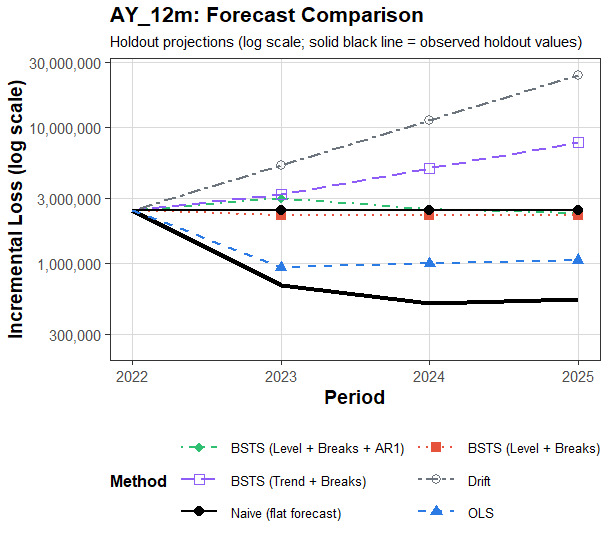
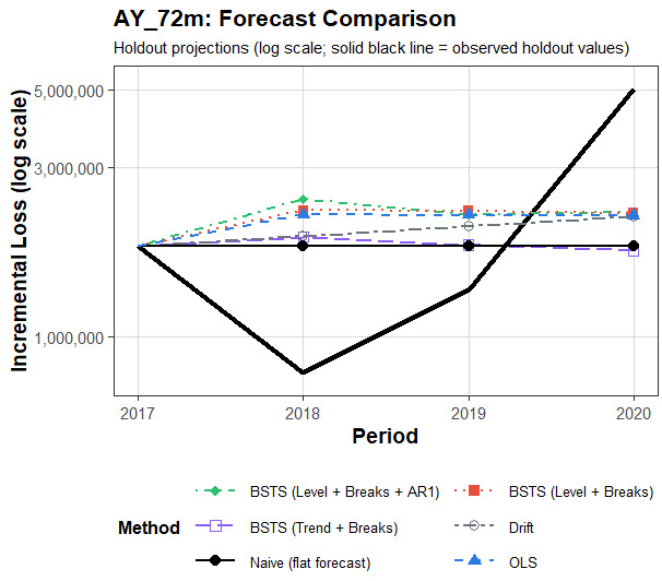
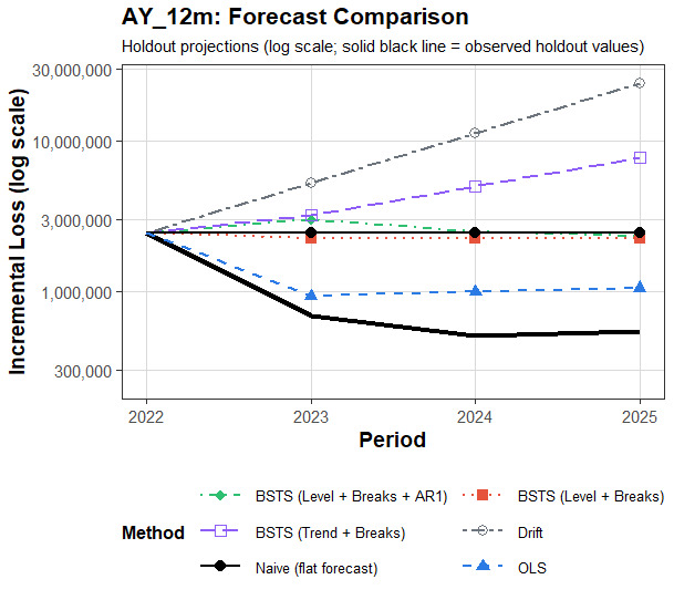
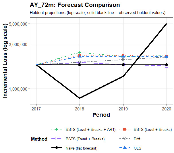
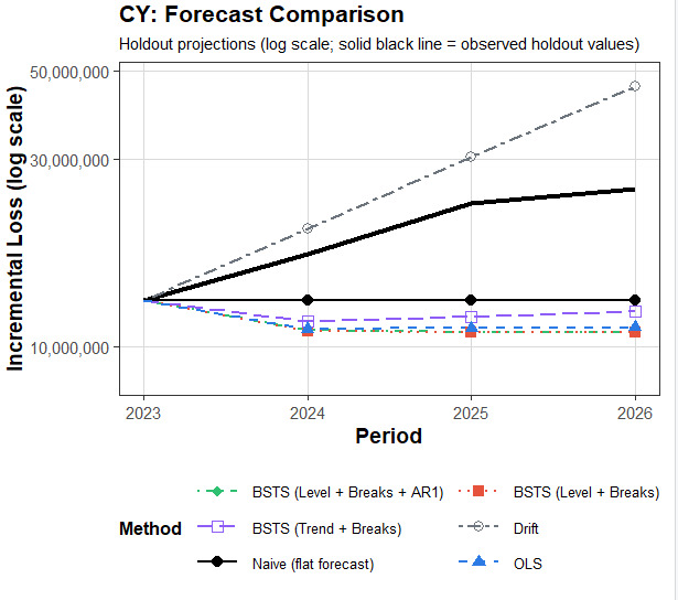
Figures 7 through 9 provide a visual comparison of forecast trajectories for each method, shown on a logarithmic scale to facilitate comparison across magnitudes and highlight relative differences in model behavior. The plots display observed values alongside out-of-sample forecasts, allowing for a qualitative assessment of how each method extrapolates recent experience. In particular, these visualizations highlight differences in the shape and stability of projected trends, as well as the extent to which models produce smooth versus more variable forecast paths—considerations that are directly relevant when selecting assumptions in a reserving analysis.

Table 2 summarizes forecast accuracy across all methods and series using MAE, MSE, and MAPE. These metrics provide a quantitative basis for comparing model performance over the holdout period, with lower values indicating improved predictive accuracy. Together, the figures and table offer complementary perspectives: The graphical results illustrate the structural behavior and intuition behind each method’s forecasts, while the tabulated metrics provide an objective comparison of their predictive performance in a setting that closely mirrors real-world actuarial forecasting decisions.

4.3.1. Results

Figure 7.Forecast accuracy summary of BSTS versus standard methods for AY_12m.

Figure 8.Forecast accuracy summary of BSTS versus standard methods for AY_72m.

Figure 9.Forecast accuracy summary of BSTS versus standard methods for CY.

4.3.2. Analysis and interpretation—Experiment 2

The forecasting results show that BSTS performs comparably to benchmark methods, with performance varying by series characteristics. No single method consistently dominates across all time series, and differences in forecast accuracy are generally modest.

For more stable and mature series, such as AY₇₂_m, BSTS produces smooth and consistent forecasts that track recent experience without overreacting to short-term fluctuations. In such settings, its performance is broadly comparable to simple trend-based approaches, reflecting the relatively stable underlying structure.

In earlier development series, such as AY₁₂_m, where volatility is higher and recent movements are less stable, simpler benchmark methods, such as the naïve model, which holds the latest observed value constant, or the drift model, which extrapolates the most recent change forward, often perform similarly or, in some cases, slightly better. In these cases, BSTS behaves as a smoothed extrapolation of recent experience, which may lag rapid changes but provides more stable projections overall.

For the CY series, which aggregate multiple development periods and exhibit more complex dynamics, BSTS performs competitively and in some cases shows improved stability relative to simpler methods. However, gains in accuracy remain modest, and results are sensitive to the underlying structure of the series.

Overall, the results suggest that while BSTS is capable of producing reasonable forecasts, it does not consistently outperform simpler approaches in this setting. Its primary value lies not in superior predictive accuracy, but in its ability to provide a structured decomposition of the series that supports interpretation alongside forecasting.

4.4. Experiment 3: Perturbation and attribution analysis using BSTS decomposition

This section presents the results of the perturbation-based attribution analysis described in the experimental design, with the goal of evaluating how BSTS allocates observed changes across its structural components. As in the prior experiments, results are shown for representative time series including early-development accident-quarter (AQ_3m), mature-development accident-quarter (AQ_18m), and calendar-quarter (CQ) series. Complete results for all analyzed series are provided in Appendix C (Experiment 3).

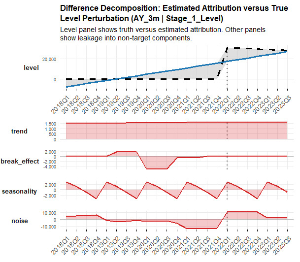
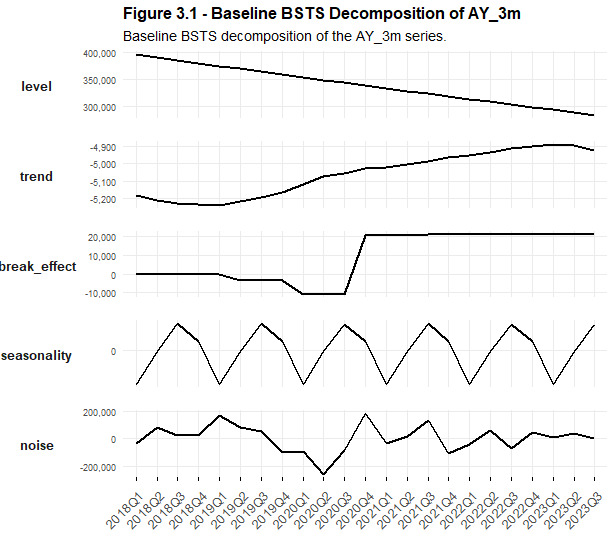
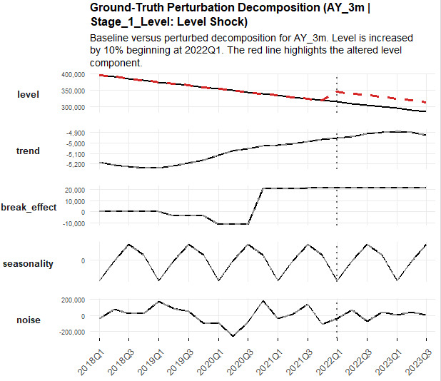
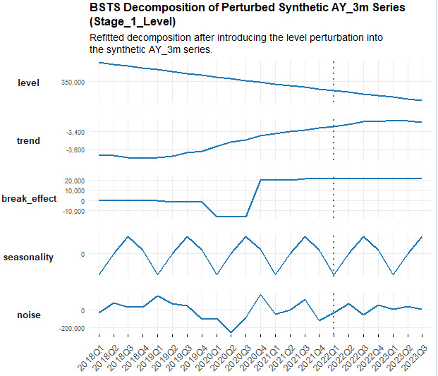
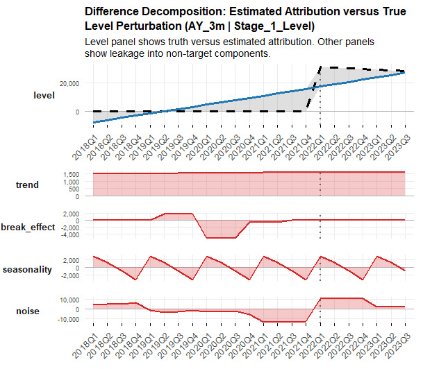
For each case, Figures 10 through 13 show the sequential reconstruction of the “observed” time series (AQ_3m) following perturbation, along with the corresponding BSTS decomposition after refitting the model. The visualizations highlight how the introduced perturbations—applied to a single component at a time within the baseline decomposition—are reflected in the estimated components upon reestimation. In particular, these plots allow for a qualitative assessment of whether the model attributes the induced variation to the intended component or distributes it across multiple components. Because three independent replicates of each perturbation type are generated, the figures reflect representative outcomes rather than any single realization, providing a more stable view of model behavior.

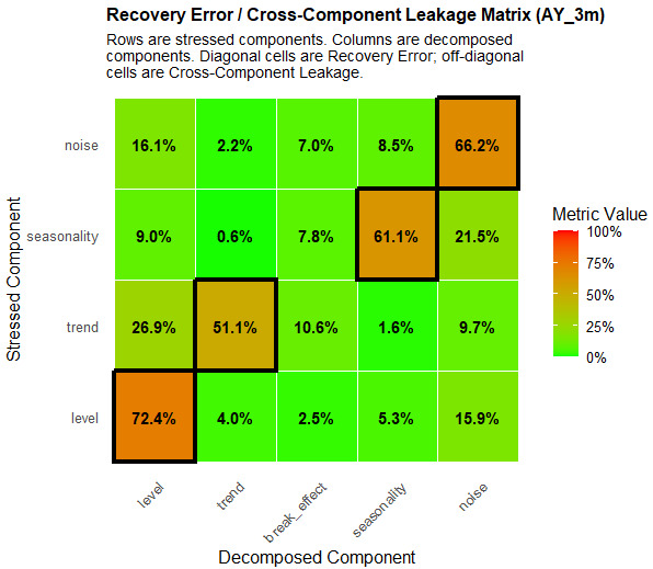
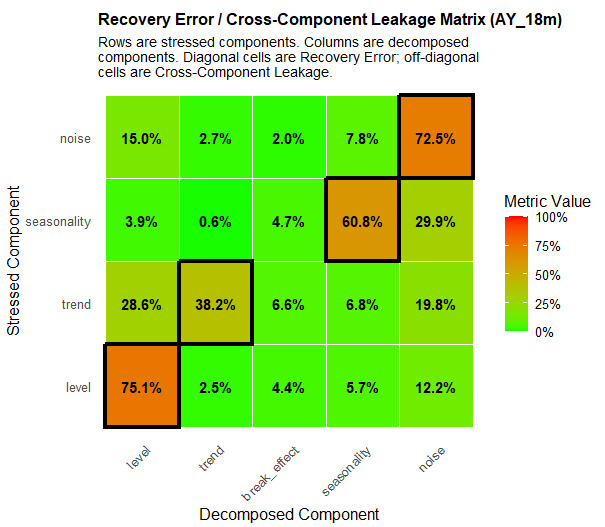
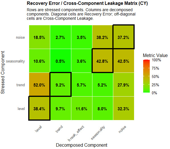
In addition to the visual results, a summary heat map is presented at the end of this section, along with its corresponding tabular representation (in Appendix C). This summary aggregates results across all series, components, and perturbation types, and reports normalized percentages that quantify how perturbations to a given component are attributed across all estimated components.

4.4.1. Results

Figure 10.Baseline fit of AQ_3m using BSTS as “ground-truth” representation of time series to which perturbations will be applied.

Figure 11.Modified BSTS fit with level perturbation added beginning in 2022Q1.

Figure 12.BSTS decomposition of AQ_3m level-perturbed baseline into components.

Figure 13.Difference decomposition—the remaining “signal” when the true level-perturbed BSTS baseline (Figure 11) is subtracted from the BSTS fit to the perturbed baseline; shows the attribution of the level shift across different components (dashed line = true perturbation).

Figure 14.Matrix summary of recovery error and cross-component leakage across all component stressors for AQ_3m.

Figure 15.Matrix summary of recovery error and cross-component leakage across all component stressors for AQ_18m.

Figure 16.CY trend/inflation “shock” manifests as a level shift/break effect (for maturities greater than three months) and an equivalent trend in AY space.

4.4.2. Analysis and interpretation—Experiment 3

The results of Experiment 3 illustrate how BSTS represents structural changes when a known perturbation is introduced, focusing on how the induced signal is distributed across components rather than whether it is recovered uniquely. The percentage attribution framework highlights how the model allocates the perturbation across level, trend, seasonal, break, and noise components.

Across AQ series, level perturbations exhibit the strongest and most consistent attribution. A majority of the induced signal is assigned to the level component, indicating that BSTS reliably interprets step changes as shifts in the baseline. However, attribution is not exclusive, with portions of the signal distributed to trend and, in some cases, break components. This reflects the fact that a persistent level shift can also be represented as a sequence of incremental changes over time.

Trend perturbations show more diffuse attribution patterns. While a meaningful share of the signal is assigned to the trend component—particularly in more mature AQ series such as AQ₁₈_m—there is consistent allocation to level and break components. This reflects both the similarity between gradual slope changes and cumulative level adjustments in short time series and the fact that many reserving trends originate in CY processes that are not naturally aligned with the accident-year/development-year indexing structure where the distinction between trend and level is not sharply identifiable.

Seasonal perturbations are identified when the signal is sufficiently strong, but attribution is less stable across series. In several cases, seasonal effects are partially absorbed into noise or distributed across other components, particularly in shorter or more volatile AQ series. This indicates that seasonal structure is only reliably captured when it is pronounced relative to overall variability.

Noise perturbations are primarily captured within the noise component, but with observable allocation to structural components. In shorter or noisier series, random variation can resemble low-frequency structure, leading the model to partially interpret noise as level or trend.

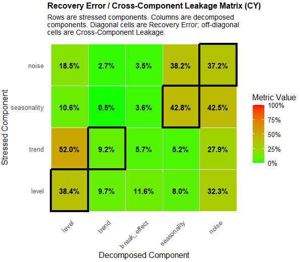
In contrast, attribution patterns in the CY series are more diffuse across all perturbation types. The induced signal is distributed more evenly across components, with less pronounced diagonal dominance. This reflects the aggregation inherent in CY series, where each observation combines contributions from multiple origin periods at different development stages, blending structural signals and reducing component-specific clarity.

Overall, the results demonstrate that BSTS does not provide a one-to-one mapping between structural perturbations and decomposed components. Instead, it produces a structured representation in which a given effect may be expressed across multiple components depending on its temporal characteristics and the context of the series. From a practical perspective, strong concentration of signal within a component provides useful diagnostic information, but cross-component allocation should be expected and incorporated into interpretation.

4.5. Experiment 4: CY perturbation decomposed in AY time series

The results of the CY perturbation extension are presented through a combination of structured visualizations and summary attribution matrices, following the same general format used in the preceding experiment. The purpose of this presentation is to illustrate how structural effects introduced in CY space are expressed when observed through AY development series of varying maturities.

Figures in this section display the impact of CY-based perturbations after transformation into AY space, expressed on a ratio-to-baseline scale to facilitate comparability across development ages and time periods. Each figure shows the evolution of the perturbed series relative to the unperturbed baseline, allowing for a clear visualization of how the imposed CY structure propagates through AY development patterns. This normalization ensures that differences in magnitude across maturities do not obscure the underlying structural effects.

For the trend (inflation) perturbation, Figure 16 illustrates how a multiplicative CY shock beginning at a fixed calendar period manifests differently across AY maturities. In particular, the visualizations highlight whether the effect appears as a gradual trend, a level shift, or a combination of both, depending on development age. For the noise perturbation, Figure 17 similarly shows how increased CY variability translates into AY space, with emphasis on whether the resulting variation exhibits persistence or remains purely stochastic.

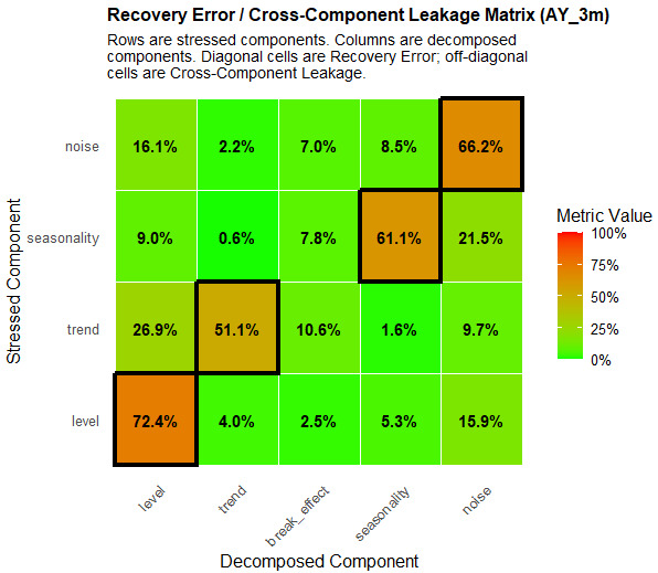
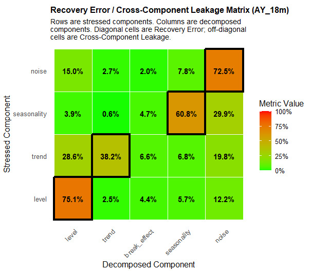
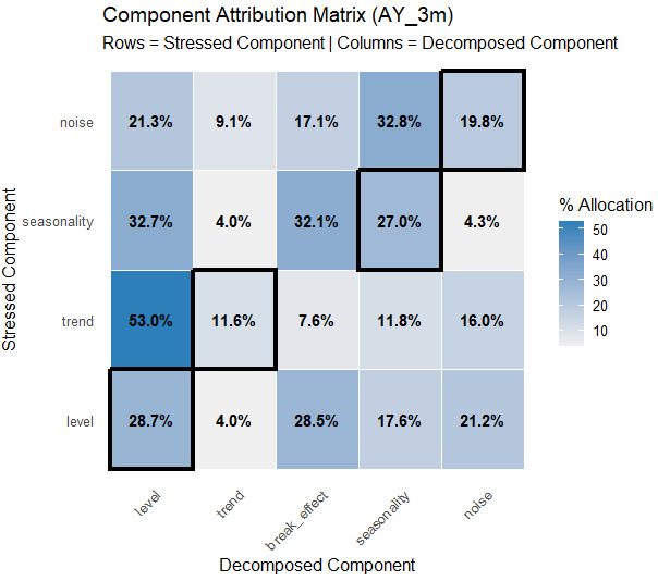
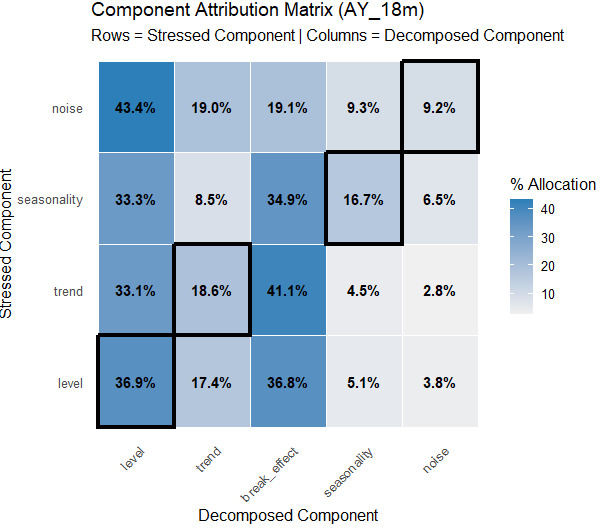
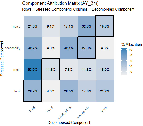
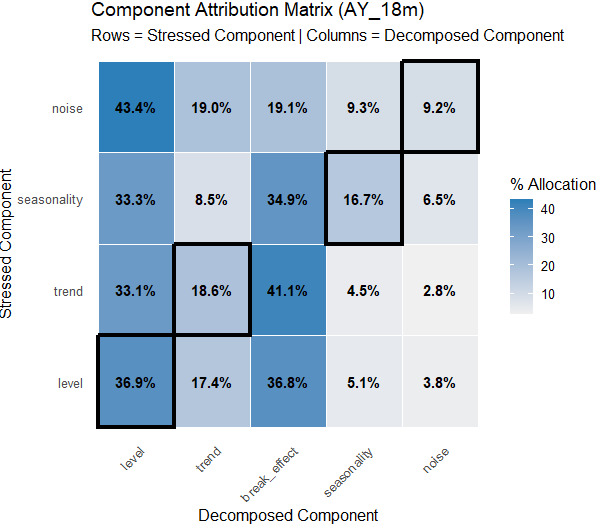
In addition to the graphical results, summary attribution matrices (Figures 18 and 19) are provided for representative AQ series (e.g., AQ_3m and AQ_18m). These matrices report normalized recovery and leakage metrics, consistent with the definitions introduced earlier, and provide a quantitative view of how CY-originating signals are distributed across BSTS components when analyzed in AY space. Together, the figures and matrices offer complementary perspectives: The visualizations provide intuition into the transformation mechanics, while the tabulated results quantify the resulting attribution behavior.

4.5.1. Results

Figure 17.CY noise shock manifests as random, nonpersistent fluctuations across all maturities, with no systematic level shift or trend in AY space.

Figure 17.CY noise shock manifests as random, nonpersistent fluctuations across all maturities, with no systematic level shift or trend in AY space.

Figure 18.Matrix summary of component attribution of CY stressors mapped to AY_3m.

Figure 19.Matrix summary of component attribution of CY stressors mapped to AY_18m.

4.5.2. Analysis and interpretation—Experiment 4

The results of Experiment 4 illustrate how structural shocks introduced in CY space are represented when mapped into AQ series and how BSTS attributes these effects across components.

A key result is that CY shocks do not translate into a single, consistent structural form in AQ space. Instead, their representation depends on development maturity. For example, whereas a CY trend shock—such as sustained inflation—manifests in early AQ maturities as a combination of an initial level shift followed by a trend, in more mature AQ series it appears closer to a persistent trend with reduced initial discontinuity. This reflects the shifting relationship between CY and AQ indexing, where the same underlying process is observed at different points along the development path.

BSTS captures this behavior through a distributed allocation of signal across components. In early AQ series, a larger share of the signal is assigned to the level and break components, reflecting the appearance of an abrupt change at the start of the series. In more mature AQ series, attribution shifts toward the trend component, consistent with a smoother evolution over time. This transition across maturities highlights how the same CY-driven effect can be represented differently depending on the temporal perspective.

Noise shocks in CY space are translated more directly into AQ noise, with the majority of the signal remaining in the noise component across maturities. However, some allocation to structural components is still observed, particularly in shorter or more volatile AQ series, where random variation may resemble low-frequency structure.

Across all perturbation types, attribution patterns remain more diffuse in CY space than in AQ series. This reflects the aggregation inherent in CY data, where each observation combines multiple origin periods and development stages, blending structural signals and reducing component-specific clarity.

From a practical standpoint, these results reinforce that structural interpretation depends on the choice of time index. Calendar-driven effects such as inflation, legal changes, or operational shifts may appear as different combinations of level, trend, and break behavior when viewed in AQ space. Accordingly, BSTS decompositions should be interpreted in the context of how the underlying data are indexed, rather than as uniquely identifying the form of the underlying process.

Conclusion

This paper examines the application of BSTS models to a central challenge in property and casualty reserving: understanding and interpreting the drivers of loss development. While traditional methods focus on estimating ultimate losses, they provide limited insight into the structural mechanisms underlying observed patterns. BSTS offers a complementary framework that decomposes loss development into interpretable components, enabling a more structured view of how losses evolve over time.

Across the experiments, BSTS is shown to capture dominant structural features such as level shifts and sustained trends and to produce forecasts that are broadly comparable to standard approaches. However, forecasting performance is not uniformly superior, and simpler methods often perform similarly, particularly in shorter or more volatile series.

The primary contribution of this work lies in the analysis of structural attribution. The results demonstrate that BSTS does not provide a one-to-one mapping between underlying processes and decomposed components. Instead, structural effects are often distributed across multiple components, reflecting the inherent non-uniqueness of decomposition in short and noisy time series.

This non-uniqueness is further illustrated through the relationship between CY and AQ representations. A single CY-driven process, such as inflation or changes in claim severity, may manifest as different combinations of level, trend, and break behavior depending on development maturity. As a result, structural interpretation depends critically on the temporal perspective through which the data are viewed.

From a practical standpoint, these findings suggest that BSTS outputs should be interpreted as structured representations of variation rather than definitive causal decompositions. Concentration of signal within a component provides useful diagnostic information, but cross-component attribution should be expected and incorporated into interpretation. In this sense, BSTS is best viewed as a tool for organizing and understanding patterns in the data, rather than for uniquely identifying their source.

Accordingly, BSTS is not a replacement for traditional actuarial methods, but a complementary framework that enhances interpretability and supports more informed judgment. It can help identify structural shifts, assess the persistence of emerging trends, and distinguish between systematic patterns and transient fluctuations. In addition, BSTS decompositions may provide a useful starting point for developing and refining reserving model structures by highlighting candidate drivers of observed development behavior.

Several directions for future research remain. Extending the framework to incorporate relationships across development periods, such as through hierarchical or multivariate models, may improve identifiability and coherence across maturities. In addition, applying the approach to longer or more granular datasets may enhance the ability to distinguish between competing structural explanations. Further work is also needed to integrate BSTS-based diagnostics into practical reserving workflows.

In summary, BSTS provides a flexible and interpretable framework for analyzing loss development. While its outputs require careful interpretation, its ability to represent and organize complex structural patterns makes it a useful addition to the actuarial tool kit.