The Value of Insurance

undefined

1. Introduction

In this paper, we provide a basis with which to measure the value of capital protection provided by insurance policies. In particular, for insurance covering low-frequency events, the value of capital protection is a significant portion of the total value of the policy. We provide an analytical framework insureds can use to compare the total value of the insurance to the premium for the insurance policy to understand whether the insurance purchase is accretive.

1.1. Commercial insurance programs

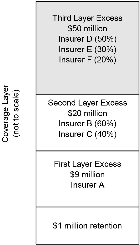
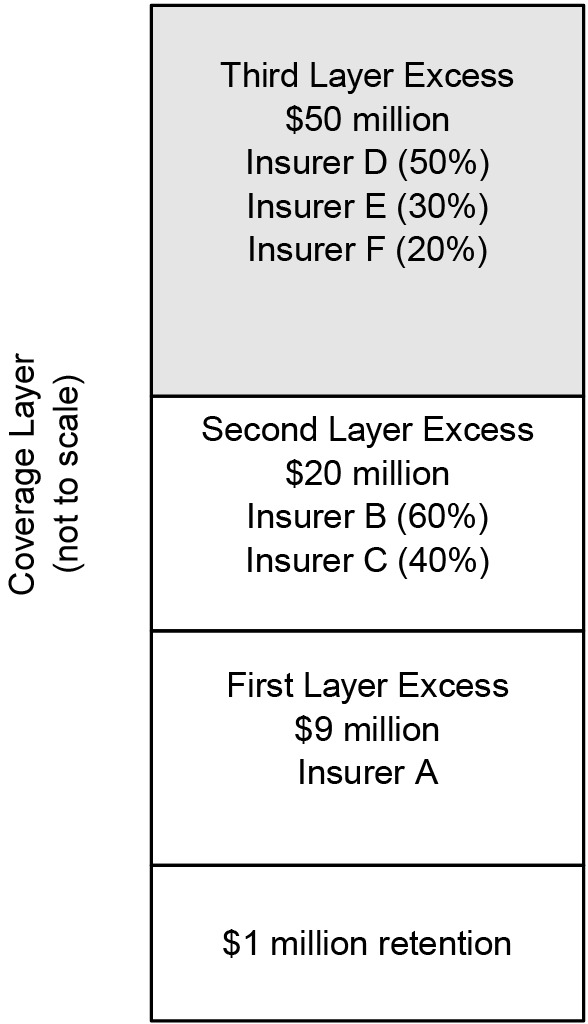
Commercial insurance programs are often depicted as towers (Figure 1). Extending this analogy, risk retained by the insured typically comprises the lowest floors of the tower. The middle floors include commercially insured working layers. High excess layer insurance resides in the penthouse. In the lower floors, the tenant pays for basic shelter (i.e., loss reimbursement), a benefit that has a tangible value. In the upper floors, the tenant pays for the view, a benefit that is not as tangible immediately but that has significant value, which we describe in this paper.

Each of the layers has a cost to it. Insurers establish premiums that are sufficient to cover claim costs and expenses and to return a profit to their shareholders.^[1] The profit provision will be proportional to the volatility of the risk.^[2] That is, the required supporting insurer capital is directly proportional to the volatility of the business. As a result, more volatile business will require additional profit to satisfy the insurer’s shareholders. Consistent with this notion, we refer to the profit provision as a capital charge in describing the cost for various insurance layers below.

• The cost of the lowest layers will have a reasonable degree of predictability. Because costs are predictable, the value of insurance is minimal, and insureds will, therefore, typically retain this risk.^[3] In our example insurance tower in Figure 1, we label this layer “$1 million retention.” The cost for these layers will principally be the expected loss and expense with a minimal, but nonzero, capital charge for volatility. There may also be frictional costs associated with risk retention, such as increased audit and actuarial fees and claims costs from legal counsel and third-party claim administrators. However, the premium also includes a provision for these services when provided by the insurer.

• The middle layers provide coverage for claims related to events that occur with a degree of regularity. The amount of claims may not be reasonably predictable in a single year but is predictable over a longer time horizon. The insurance coverage provides value to the insured by smoothing claim volatility over time. There may be multiple insurers in the higher working layers. We label these layers “First Layer Excess” and “Second Layer Excess” in the example in Figure 1.

• Insureds generally do not expect to access coverage from the highest layers. As such, from the insureds’ perspective, the most likely outcome (i.e., the mode) may be $0. The expected value of loss, however, will be nonzero, and the variance of claims in this layer for an individual insured is likely significant. Insurers providing coverage in this layer smooth claims volatility over risks and time. Over its aggregate high-excess portfolio, the individual insurer will have a non-negligible expected value and, likely, a significant variance. As a result of the need to smooth volatility across risks, there are often multiple insurers in these layers, each with a pro rata share. In Figure 1, we label this layer “Third Layer Excess.”

1.2. A personal insurance parallel

Similarly, the coverage for the loss of a residence^[4] provided by homeowners coverage principally protects the insured’s capital (i.e., personal savings). Insureds generally don’t expect a home fire in any given year (or in a multiyear period). The insured does not purchase such insurance expecting a claim payment. The value of the insurance results from the insured being able to deploy their capital (i.e., spend their income) to enjoy life’s activities, rather than setting aside that income for the unlikely home fire.

1.3. The value of insurance

The principles we present in this paper apply to all layers of insurance. It’s useful, however, to consider the value of the capital protection provided by insurance for low-frequency events as it represents a greater share of the total value as compared to insurance for events that occur more regularly. Despite lower expected claim values, premiums for this insurance can be significant.

Sometimes buyers refer to such insurance as “sleep insurance”—that is, the insurance allows the buyer to sleep at night. In this paper, we describe an approach that the buyer can use to help understand whether there is financial value^[5] to the insurance transaction.

To assess the potential financial value, we should understand that the primary benefit of this layer is not in the loss reimbursement but in the protection of capital that this layer of insurance provides to the insured.

• For commercial policies, the insured often considers the insurance in this layer as part of its capital structure rather than as an operational cost. The insurance allows the firm to deploy the capital that it would otherwise need to set aside to weather an extreme loss event.

• In addition to this protection of capital, the insurance will also reduce earnings volatility and potentially improve the firm’s attractiveness to investors.

In this paper, we quantify these benefits of insurance.

1.4. Literature search

Most research related to capital in the insurance transaction focuses on the insurer’s return on capital rather than on the protection of the insured’s capital. The limited research related to the insured’s preference focuses on utility theory (as a function of wealth), and such research is generally presented in the context of personal insurance coverages (such as homeowners).

Capital protection and wealth maximization are related concepts, and utility functions (generically) provide a basis to assess alternatives. That approach is not dissimilar to the one that we present in this paper. However, the research we present has differences:

• Whereas utility functions are typically abstract, the measurement approach we present in this paper is more specifically defined.

• Valuations based on utility theory are common in economics. In this paper, we present an actuarial view based on risk (i.e., variance) reduction.

We list the works that we reviewed in Appendix B.

1.5. Presentation outline

In this paper, we consider two primary sources of value for the insured:

• The ability to deploy capital that it otherwise would have had to set aside for an insurable event. We present our review of this source of value in Section 2.

• Reduced volatility of earnings and the resulting reduction in required return. We present our review of this source of value in Section 3.

2. Capital deployment

In this section, we describe how insurance allows the insured to deploy capital that it otherwise would need to set aside to weather a loss event. The analysis we present does not relate to the entire capital structure of the firm but rather only to that portion allocated to activities that are subject to the risk of insurable claims. Hereafter, all references to capital (which we later denote as $C$) relate to this portion of the firm’s capital structure.

To measure the value of insurance related to the firm’s ability to deploy that capital, we compare rates of return when the firm “funds” the claims risk without insurance (i.e., with reserved capital) to rates of return when the firm transfers risk using insurance.

2.1. Funding risk using capital

We first present an analysis to demonstrate conceptually why a firm would find it necessary to set aside capital. We do not intend this analysis to be a prescriptive approach for determining the amount of capital to set aside.

We use the following notation in our analysis:

• We denote deployed capital, i.e., the working capital, as $C_w$.

• We denote the maximum probable claim amount as $X_\text{max}$.

• We denote the risk-free rate as $r_f$.

In our review, we assume the following:

• There is a fixed amount of capital, $C$, available to the firm.

• The firm requires a minimum level of capital, $C_{\text{min}}$, to continue as a going concern.

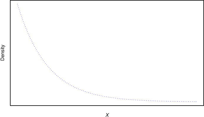
• The firm is subject to the loss events that result in aggregate claim amounts, $X$. We present the distribution of claim amounts in Figure 2.^[6]

• For simplicity, we assume information symmetry with respect to $X$. That is, the insurer and the insured use the same distribution for $X$.

• The scale of $X$ is a function of $C_w$.

• The firm has an enterprise risk management (ERM) strategy underlying its capital allocation. Its ERM strategy dictates that it can absorb a claim at the $p^{th}$ percentile of the distribution of $X$, which we denote as $X_p$.

• The firm is able to generate a rate of return on capital^[7] of $r_c$. For purposes of determining the value of insurance, we use a simplifying assumption that $r_c$ is fixed. That is, $E(r_c)=r_c$ and $Var(r_c)=0$.

• We assume that the firm can capture expected costs for both premiums and retained loss through pricing of its products. That is, we view these as operational costs that do not require capital segregation, and the higher-cost option does not marginally erode capital.

2.2. Rate of return without insurance

When a firm retains risk, it must allocate capital for that risk. The firm may allocate that capital with or without a formal analysis as to the amount of capital that it must set aside. In this section, we present an example of actions that a firm with an ERM strategy may adopt^[8] when faced with risk.

The firm’s ERM strategy requires it to reserve capital for the possibility that it experiences a capital depletion event (i.e., a loss). We denote this reserve as $C_{x}$ to indicate that the reserve is a segregation of capital to absorb realizations of $X$.

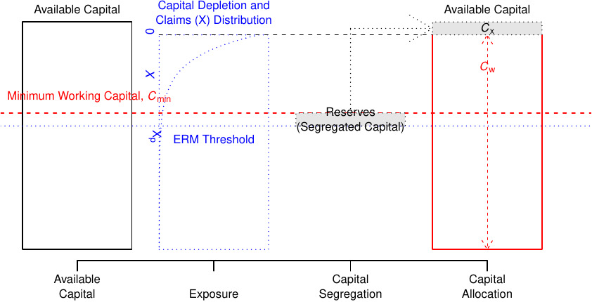
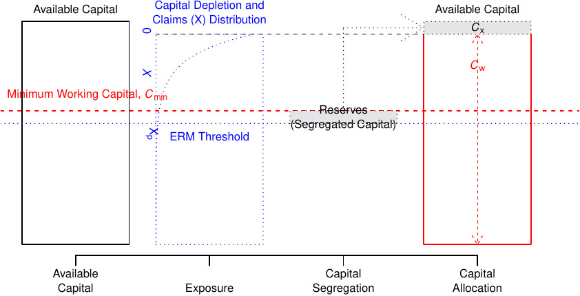
We present this capital allocation approach in Figure 3 and offer the following extended comments. We refer to the sections of Figure 3 as “blocks,” with the names below each block.

• The first block represents the capital available to the firm.

• The firm must maintain the minimum working capital denoted as $C_{\text{min}}$ to continue operations.

• The firm has exposure to capital depletion events, $X$, as presented in Figure 2. This “Exposure” block is the same as Figure 2 rotated clockwise and scaled to the level of working capital, $C_w$ (described below).

• The firm’s ERM strategy supports business continuity for capital depletion events (i.e., claims or other loss events) of size $X_p$. Since $X_p$ is greater than $C - C_\text{min}$, the firm will need to set aside capital so that it can maintain $C_{\text{min}}$ if it were to experience a claim of $X_p$. The “Capital Segregation” block presents the amount that would need to be set aside.

• The final block demonstrates the need to segregate capital. We present the final capital structure in the “Capital Allocation” block. The firm is able to deploy capital of $C_w$ (since it needed to set aside $C_x$). If it experiences a loss of $X_p$ (which, as noted, is from a claim distribution scaled to $C_w$), then its working capital would fall below $C_{\text{min}}$. The segregated capital, $C_x$, restores remaining working capital, $C_w - X_p$, to $C_{\text{min}}$.

  We place the segregated capital, $C_x$, at the top of the capital allocation block. This presentation should not imply that the $C_x$ is accessed first in the case of claim. Rather, in the event of a claim of size $X_p$, the firm would first deplete the working capital to $C_{min}$ and then fund the remainder of the claim with $C_x$. (Alternatively and equivalently, the firm would deplete capital below $C_{min}$ and then replenish using the set-aside capital, $C_x$.) We use this presentation to support the understanding of segregation of capital rather than the order of access.

Using the naught superscript to represent this “without insurance” base case, the rate of return is as follows:

$$R^0 = \dfrac{r_c \times C_{w}^{0} + r_f \times C_{x}^{0} - X}{C}.\tag{1}$$

The numerator is the sum of the return on working capital and the return on the reserve (segregated capital) less the value of the claim amount. The inclusion of the random variable $X$ indicates that the firm’s return is a function of the realized value of the loss event.

Taking expectations, we have

$$E[R^0] = \dfrac{r_c \times C_{w}^{0} + r_f \times C_{x}^{0} - E[X]}{C}.\tag{2}$$

2.3. Rate of return with insurance

The firm may alternatively elect to purchase insurance to cover a portion of the cost of the loss event. We develop that rate of return in this section.

We use the following notation in our rate-of-return equation:

• $X_\text{ret}$ represents the portion of the distribution of claims values that the firm retains. We allow $X_\text{ret}$ to vary between 0 (in which the firm fully transfers the risk) and $X_\text{max}$ (equal to the no-insurance case). We observe that if the retention will not reduce capital below $C_{\text{min}}$, i.e., if $X_\text{ret} < (C_\text{w} - C_\text{min})$, then no capital would need to be set aside to cover loss events, i.e., $C_x = 0$. If this were the case, then the firm could view the insurance costs as an operational expense, which is evident with this substitution into Equation (2).

• We use superscript $I$ to represent the insurance case. $P^{I}$ represents the premium (in the insurance case), and $C_{x}^{I}$ represents the capital that would be set aside to pay claims. This notation is consistent with the $C_{x}^{0}$ notation that we use for capital in the no-insurance case. (They both represent approaches to fund risk.)

The rate of return in the insurance case is as follows:

$$R^I = \dfrac{r_c \times (C - C_{x}^{I}) + r_f \times C_{x}^{I} - X_\text{ret} - P^{I}}{C}.\tag{3}$$

However, we assume $r_c > r_f$ as without this condition there is no economic value to the firm’s existence. As such, the rational firm purchases insurance such that it need not set aside any capital. Therefore, $C_{x}^{I} = 0$. Simplifying Equation (3) we have

$$R^I = \dfrac{r_c \times C + - X_\text{ret} - P^{I}}{C}.\tag{4}$$

Taking expectations results in the following:

$$E[R^I] = \dfrac{r_c \times C - E[X_\text{ret}] - P^{I}}{C}.\tag{5}$$

The interpretation of the numerator is intuitive. The firm earns a rate of return, $r_{c}$, on its initial capital. We then subtract the expected retained claims and the premium. Also, and importantly, the firm is able to deploy all of its capital, $C$, which earns a rate of return, $r_c$, in exchange for paying a premium, $P^I$.

We reorder terms to support the value analysis:

$$E[R^I] = \dfrac{-P^{I} + r_c \times C - E[X_\text{ret}]}{C}.\tag{6}$$

2.4. The value of capital deployment

We now have a construct to determine the capital deployment value provided by the premium. We do so by calculating the premium that results in an equivalent rate of return with and without insurance.

$$\small{\begin{aligned} E[R^I] &= E[R^0], \notag\\ \dfrac{-P^{I} + r_c \times C - E[X_\text{ret}]}{C} &= \dfrac{r_c \times C_{w}^{0} + r_f \times C_{x}^{0} - E[X]}{C},\notag\\ -P^{I} + r_c \times C - E[X_\text{ret}] &= r_c \times C_{w}^{0} + r_f \times C_{x}^{0} - E[X],\notag\\ -P^{I} &= r_c \times (C_{w}^{0} - C) + r_f \times C_{x}^{0} + E[X_\text{ret}] - E[X],\notag\\ P^{I} &= r_c \times (C - C_{w}^{0}) - r_f \times C_{x}^{0} + (E[X] - E[X_\text{ret}]), \notag\\ P^{I} &= r_c \times C_{x}^{0} - r_f \times C_{x}^{0} + E[X_\text{ins}],\notag\\ P^{I} &= (r_c - r_f ) \times C_{x}^{0} + E[X_\text{ins}]. \end{aligned}\tag{7}}$$

The interpretation of Equation (7) is intuitive. The premium provides two sources of value:

• The excess return on capital that need not be segregated if the firm purchases insurance

• The expected value of insured claims

3. Risk adjustment to required return

The second source of value results from the reduction in the volatility of returns for insurance buyers. The value creation results from the lower required return for firms with reduced earnings volatility. The theory behind the Sharpe ratio provides a framework to measure this value.

The Sharpe ratio relates the risk premium required (numerator) to return volatility (denominator). More specifically, it represents the risk premium required for every unit of volatility. The common use of the Sharpe ratio is to support comparative investment decisions.

We recognize the assumption of the normality of returns underlying the Sharpe ratio. In this paper, we are not validating the assumptions underlying the Sharpe ratio. Rather, we are using the intuitive concepts underlying the ratio, which are the same concepts as we discussed related to the profit provision in insurance to evaluate the purchase of insurance.

$$\text{Sharpe ratio} = \frac{E(R)-r_f}{\sigma_{R}}.$$

As we did in measuring the value through capital deployment, we first calculate the Sharpe ratio without insurance (i.e., the base case) and then compare that to the Sharpe ratio for the insurance buyer.

As we are concerned with the marginal value created by the insurance transaction, we can calculate $E(R)$ and $Var(R)$ in this section under the following assumptions:

• The risk-free rate, $r_f$, is fixed.

• $X$ and $r_c$ are independent.

3.1. Sharpe ratio without insurance

As with the discussion in Section 2, we use the naught superscript to represent the base case.

Recall that we developed the expected rate of return in Section 2.2. We rewrite Equation (2) thusly:

$$\begin{aligned} R^{0} &= \dfrac{r_c \times C_w^{0} + r_f \times C_{x}^{0} - X}{C}, \notag\\ E[R^{0}] &= E\left[\dfrac{r_c \times C_w^{0} + r_f \times C_{x}^{0} - X}{C}\right]\notag\\ &=\dfrac{(C-C_{x}^{0})\times r_c + r_f \times C_{x}^{0} - E[X]}{C}. \end{aligned}\tag{8}$$

We start with Equation (1) and develop the variance of returns under the simplifying conditions described at the beginning of this section.

$$\begin{aligned} Var[R^{0}] &= Var\left[\dfrac{r_c \times C_w^{0} + r_f \times C_{x}^{0} - X}{C}\right]\notag\\ &=\dfrac{Var(X)}{C^2}.\notag \end{aligned}$$

We can now calculate the Sharpe ratio without insurance.

$$\small{ \begin{aligned} \text{Sharpe ratio}^0 &=\frac{E(R_0)-r_f}{\sigma_{R_0}} \notag\\ &= \dfrac{\left[\dfrac{(C-C_{x}^{0})\times r_c + r_f \times C_{x}^{0} - E[X] - r_f \times C}{C}\right]}{\left[\dfrac{Var(X)}{C^2}\right]^{0.5}}\notag\\ &= \frac{(C-C_{x}^{0})\times (r_c-r_f) - E[X]}{SD(X)}. \end{aligned}\tag{9} }$$

3.2. Sharpe ratio with insurance

We can also calculate the Sharpe ratio for the insurance buyer, using the superscript $I$ to represent this case. As with the no-insurance case, we start with Equation (6) from Section 2.3:

$$E[R^I] = \dfrac{-P^{I} + r_c \times C - E[X_\text{ret}]}{C}. \nonumber$$

We start with Equation (4) and develop the variance under the simplifying conditions described at the beginning of this section.

$$\begin{aligned} R^I &= \dfrac{r_c \times C + - X_\text{ret} - P^{I}}{C}, \\ Var[R^{I}] &= Var\left[\dfrac{r_c \times C - X_\text{ret} - P^{I}}{C}\right],\\ Var[R^{I}] &=\dfrac{Var(X_\text{ret})}{C^2}. \end{aligned}$$

Now we calculate the Sharpe ratio under the insurance case:

$$\begin{aligned} \text{Sharpe ratio}^I &= \dfrac{E(R_I)-r_f}{\sigma_{R^0}} \notag\\ &=\dfrac{\left[\dfrac{-P^{I} + r_c \times C - E[X_\text{ret}] - C \times r_f}{C}\right]}{\left[\dfrac{Var(X_{ret})}{C^2}\right]^{0.5}} \notag\\ &=\dfrac{C\times (r_c-r_f)-P^{I} - E[X_{ret}]}{SD(X_{ret})}. \end{aligned}\tag{10}$$

3.3. Complete value creation equation

The insurance purchase creates value when it results in an increase in the Sharpe ratio. We can use Equation (9) and Equation (10) to calculate the maximum premium that results in value creation. We present that equation below.

$$\begin{aligned} \nonumber \text{Sharpe ratio}^I &> \text{Sharpe ratio}^0,\\ \nonumber \dfrac{C\times (r_c-r_f)-P^{I} - E[X_\text{ret}]}{SD(X_\text{ret})} &> \dfrac{(C-C_{x}^{0})\times (r_c-r_f) - E[X]}{SD(X)},\\ \nonumber \cdots &> \cdots\\ \end{aligned}$$

$$\begin{align} P_{I} &< E[X_\text{ins}] + C_{x}^{0} \times (r_c-r_f) \\&\quad+ \left[1 - \dfrac{SD(X_\text{ret})}{SD(X)} \right] \\&\quad\times \left[E[X] - C_{w}^{0} \times (r_c-r_f)\right]. \end{align} \tag{11}$$

We present the complete algebraic derivation in Appendix A.

The interpretation of Equation (11) is more difficult than that posed by Equation (7).

• The first two terms of the right-hand side are the same as those included in Equation (7). Then, recognizing that $SD(X_\text{ret})<SD(X)$, we’ll recognize that $\left[1 - \dfrac{SD(X_{ret})}{SD(X)}\right]$ will be between 0 and 1. We also expect the $E[X] - C_{w}^{0} \times (r_c-r_f)$ term to be positive as we’d expect $r_c-r_f$ to be positive. As such, the final term represents the additional (positive) value created by the reduction in volatility.

• We recognize that as the volatility insured rises, the volatility retained reduces. In this case, $\left[1 - \dfrac{SD(X_{ret})}{SD(X)}\right]$ will increase and the value of the insurance will also increase.

• If all the risk is retained, i.e., $SD(X_\text{ret}) = SD(X)$, then Equation (11) reduces to Equation (7).

• If all the risk is insured, i.e., $SD(X_\text{ret}) = 0$ and $C_{x}^{0} = 0$, then the value of insurance is greater than one but less than two times the expected loss.

We refer to Equation (11) as the complete value creation equation, since it includes both sources of value. We should not find this surprising since the Sharpe ratio includes expected returns in its numerator and risk/volatility in the denominator.

4. Conclusion and summary

Through the analysis presented in the paper, we have developed a measurement of two sources of value from the insurance transaction.

• The value that results from the ability of the firm to deploy additional capital:

$$\begin{aligned} E[X_\text{ins}] + C_{x}^{0} \times (r_c-r_f). \end{aligned}\tag{12}$$

When premium amounts satisfy Equation (7), the insurance transaction will be accretive to the rate of return.

• The value created through the reduced earnings expectations that result from the reduction in volatility:

$$\begin{aligned} \left[1 - \dfrac{SD(X_\text{ret})}{SD(X)} \right] \times \left[E[X] - C_{w}^{0} \times (r_c-r_f)\right]. \end{aligned}\tag{13}$$

When premium amounts do not satisfy Equation (7) but satisfy Equation (11), the insurance transaction will not be accretive to the rate of return. However, the reduction in the rate of return will be less than the reduction in the rate of return demanded by the shareholder due to the reduced volatility.

When premium amounts do not satisfy either Equation (7) or Equation (11), then the insurance transaction does not add financial value. However, it may still provide value in supporting a restful night’s sleep.

Appendices

A. Algebraic Derivation of Complete Value Creation Equations

$$\small{ \begin{aligned} \nonumber \text{Sharpe ratio}^I &> \text{Sharpe ratio}^0,\\ \nonumber \dfrac{C\times (r_c-r_f)-P^{I} - E[X_\text{ret}]}{SD(X_\text{ret})} &> \dfrac{(C-C_{x}^{0})\times (r_c-r_f) - E[X]}{SD(X)},\\ \nonumber C\times (r_c-r_f)-P^{I} - E[X_{ret}] &> \dfrac{SD(X_\text{ret})}{SD(X)} \left[ (C-C_{x}^{0})\times (r_c-r_f) - E[X] \right],\\ \nonumber -P^{I} &> \dfrac{SD(X_{ret})}{SD(X)} \left[ (C-C_{x}^{0})\times (r_c-r_f) - E[X] \right] \\&\quad+ E[X_\text{ret}] - C\times (r_c-r_f). \end{aligned} }$$

We can rearrange the terms on the right-hand side related to $E[X]$ as follows, noting that $E[X] = E[X_\text{ret}] + E[X_\text{ins}]$:

$$\begin{aligned} & E[X_{ret}] - \dfrac{SD(X_\text{ret})}{SD(X)} E[X] \notag\\ & E[X] - E[X_\text{ins}] - \dfrac{SD(X_\text{ret})}{SD(X)} E[X]\notag\\ & -E[X_{ins}] + \left[1 - \dfrac{SD(X_{ret})}{SD(X)}\right] E[X]\notag\\ & \left[1 - \dfrac{SD(X_\text{ret})}{SD(X)}\right] E[X] - E[X_\text{ins}]\notag\\ &\left[\dfrac{SD(X_{ret})}{SD(X)} - 1\right] (-E[X]) - E[X_\text{ins}]\notag \end{aligned}$$

Now, we rearrange the terms on the right-hand side related to $C$:

$$\small{ \begin{aligned} \nonumber \dfrac{SD(X_\text{ret})}{SD(X)} (C-C_{x}^{0})\times (r_c-r_f) &- C\times (r_c-r_f)\\ \nonumber \left[\dfrac{SD(X_\text{ret})}{SD(X)} - 1 \right] \times C \times (r_c-r_f) &- \dfrac{SD(X_\text{ret})}{SD(X)} \times C_{x}^{0} \times (r_c-r_f)\\ \nonumber &+1 \times C_{x}^{0} \times (r_c-r_f)\\ \nonumber &-1 \times C_{x}^{0} \times (r_c-r_f)\\ \nonumber \left[\dfrac{SD(X_{ret})}{SD(X)} - 1 \right] \times C \times (r_c-r_f) &- \left[\dfrac{SD(X_{ret})}{SD(X)} - 1\right] \times C_{x}^{0} \times (r_c-r_f)\\ \nonumber &-1 \times C_{x}^{0} \times (r_c-r_f)\\ \nonumber \left[\dfrac{SD(X_\text{ret})}{SD(X)} - 1 \right] \times (C - C_{x}^{0}) \times (r_c-r_f) &-1 \times C_{x}^{0} \times (r_c-r_f)\\ \nonumber \left[\dfrac{SD(X_\text{ret})}{SD(X)} - 1 \right] \times (C - C_{x}^{0}) \times (r_c-r_f) &-C_{x}^{0} \times (r_c-r_f)\\ \nonumber \left[\dfrac{SD(X_\text{ret})}{SD(X)} - 1 \right] \times C_{w}^{0} \times (r_c-r_f) &-C_{x}^{0} \times (r_c-r_f) \end{aligned}}$$

Combining both components of the right-hand side, we have

$$\small{ \begin{aligned} \nonumber -P_{I} &> \left[\dfrac{SD(X_\text{ret})}{SD(X)} - 1\right] \times \left[C_{w}^{0} \times (r_c-r_f) - E[X]\right] - E[X_\text{ins}] - C_{x}^{0} \times (r_c-r_f),\\ \nonumber P_{I} &< E[X_\text{ins}] + C_{x}^{0} \times (r_c-r_f) - \left[\dfrac{SD(X_\text{ret})}{SD(X)} - 1\right] \times \left[E[X] - C_{w}^{0} \times (r_c-r_f)\right],\\ \nonumber P_{I} &< E[X_\text{ins}] + C_{x}^{0} \times (r_c-r_f) + \left[1 - \dfrac{SD(X_\text{ret})}{SD(X)} \right] \times \left[E[X] - C_{w}^{0} \times (r_c-r_f)\right].\\ \end{aligned} }$$

B. Literature review

We identified and reviewed the following papers in our literature review. As noted, these papers focused on the return on the insurer’s capital rather than the value of capital preservation for the insured.

Macalaster, Spencer. 2015. “Insurance as a Form of Capital.” Insurance Journal, January 12. https://www.insurancejournal.com/magazines/mag-closingquote/2015/01/12/353262.htm. Macalaster described the issue conceptually but without measurement and does not mention the role of the actuary in establishing reserves.

Arrow, Kenneth Joseph. Essays in the Theory of Risk Bearing. Markham, 1971. Arrow’s theorem is the cornerstone of the application of expected utility theory in insurance.

Raviv, Artur. 1979. “The Design of an Optimal Insurance Policy.” American Economic Review 69 (1): 84–96. https://www.jstor.org/stable/1802499. Raviv used expected utility theory to measure value for an insured.

Gollier, Christian. 1996. “Optimum Insurance of Approximate Losses.” Journal of Risk and Insurance 63 (3): 369–80. https://doi.org/10.2307/253617. Gollier also used expected utility theory to optimize insured retentions.

Yaari, Menahem E. 1987. “The Dual Theory of Choice under Risk.” Econometrica 55 (1): 95–115. https://doi.org/10.2307/1911158. In this paper, Yaari presented the modification of expected utility theory.

Konrad, Kai A., and Stergios Skaperdas. 1993. “Self-Insurance and Self-Protection: A Nonexpected Utility Analysis.” Geneva Papers on Risk and Insurance Theory 18 (2): 131–46. http://www.jstor.org/stable/41953283. Konrad and Skaperdas used rank-dependent expected utility preferences to measure value for an insured.

Courbage, Christophe. 2001. “Self-Insurance, Self-Protection, and Market Insurance within the Dual Theory of Choice.” Geneva Papers on Risk and Insurance Theory 26 (1): 43–56. https://doi.org/10.1023/A:1011212324117. Courbage used dual theory to measure value for an insured.

Merz, Michael, and Mario V. Wüthrich. 2014. “Demand of Insurance under the Cost-of-Capital Premium Calculation Principle.” Risks 2 (2): 226–48. https://doi.org/10.3390/risks2020226. Merz and Wüthrich used a risk premium approach to measure value for an insured.

Bernard, Carole, Xue Dong He, Jia-An Yan, and Xun Yu Zhou. 2012. “Optimal Insurance Design under Rank-Dependent Expected Utility.” Available at SSRN: https://dx.doi.org/10.2139/ssrn.1883519. Bernard et al. used rank-dependent expected utility theory to measure value for an insured, too.

Laury, Susan K., Melayne Morgan Mcinnes, and J. Todd Swarthout. 2009. “Insurance Decisions for Low-Probability Losses.” Journal of Risk and Uncertainty 39: 17–44. https://doi.org/10.1007/s11166-009-9072-2. Laury et al. used experimental evidence to show individuals’ underinsure decision for low-probability, high-loss events.

Kunreuther, Howard, and Mark Pauly. 2004. “Neglecting Disaster: Why Don’t People Insure Against Large Losses?” Journal of Risk and Uncertainty 28 (1): 5–21. https://www.jstor.org/stable/41761127. Used utility theory to show why individuals don’t insure against low-probability and high-loss events.

---

1. Principles of insurer pricing are not within the scope of this paper. However, it will be helpful to recognize that shareholders will require a higher return for layers with greater volatility.

2. Greater volatility increases the notional capital assigned to support the risk, which increases the absolute return required for the contract.

3. The insured may realize value though specialized risk or claims management services provided by the insurer.

4. Homeowners policies provide additional coverages beyond the loss of a residence.

5. That is, the value beyond the restful night of sleep.

6. This is an illustrative claim distribution that we present to support further development of value measurement.

7. The generic reference here is to capital deployed to support operations.

8. We recognize that not all firms will allocate capital using this type of analysis.