The Negative Binomial Chain Ladder: A Full Likelihood Model for Claim Count Reserving

1. Introduction

Claims reserving is a central task in non-life insurance (see Taylor 2000; England and Verrall 2002, for textbook treatments). At each valuation date, insurers must estimate the liabilities associated with claims that have occurred but are not yet fully settled. These liabilities include both reported but not settled claims and incurred but not reported claims. While micro-level models can analyze the development of individual claims, macro-level reserving techniques remain dominant in practice due to their simplicity, transparency, and robustness.

Among macro-level methods, the chain ladder (CL) technique is by far the most widely used. Its appeal lies in its deterministic structure, where development factors are estimated from historical runoff triangles and applied multiplicatively to project future development. Despite its practical importance, the classical CL method lacks a coherent probabilistic foundation. It provides point estimates but no likelihood, and its stochastic extensions rely on assumptions that do not always align with the underlying claim process.

Two prominent stochastic extensions are the Mack model (Mack 1993; 1994) and the overdispersed Poisson (ODP) framework (Renshaw and Verrall 1998; England and Verrall 2002). The Mack model specifies only conditional first and second moments of the cumulative claims and does not assume a full probability distribution; prediction uncertainty is obtained from analytic mean-squared-error formulas rather than from a predictive distribution. The ODP model provides a quasi-likelihood interpretation but relies on a variance structure of the form \(\text{Var}(N_{i,j}) = \phi\, \text{E}[N_{i,j}]\), which may not reflect the true variability in the data. Its predictive distribution is typically obtained via residual resampling (England and Verrall 2002), which introduces additional assumptions and may not be fully consistent with the underlying claim process.

Recent work has independently pursued full-likelihood negative binomial models for count triangles. Nieto-Barajas and Targino (2026) propose Bayesian negative binomial models whose primary contribution is to relax the independence assumption across development years via moving-average dependence sequences with negative binomial marginals. Our aims are complementary but distinct: We work in a frequentist generalized linear model (GLM) framework. Rather than modeling cross-period dependence, we derive the negative binomial from a micro-level Poisson–gamma arrival process. This derivation allows us to determine the identification status of \(\kappa\) as a cell-level dispersion parameter (Remark 2) and recover the classical chain ladder point estimates exactly in the Poisson limit.

1.1. Contribution

This paper develops a negative binomial–chain ladder (NB-CL) model that provides a full likelihood for the CL method. While likelihood-based formulations of the chain ladder method exist in the literature (Renshaw and Verrall 1998; Verrall 2000), they typically treat overdispersion as a statistical nuisance parameter without structural interpretation.

The key contribution of this paper is a micro-level derivation showing that the negative binomial distribution arises naturally from a Poisson–gamma construction. Claims in cell \((i,j)\) arrive according to a Poisson process where the rate carries a multiplicative gamma shock, \(N_{i,j} \mid \varepsilon_{i,j} \sim \mathrm{Poisson}(\exp(\alpha_i)\, w_j\, \varepsilon_{i,j})\) with \(\varepsilon_{i,j} \sim \mathrm{gamma}(\kappa, \kappa)\) independent across cells. Marginalizing over the latent shock yields a negative binomial distribution for incremental counts.

This derivation gives the dispersion parameter \(\kappa\) a structural interpretation as the variability of cell-level claim-generating conditions (i.e., period-specific environment shocks around the systematic accident-year and development structure), rather than as an ad hoc overdispersion adjustment, and the constancy of \(\kappa\) across cells is the assumption of a homogeneous shock distribution.

Heterogeneity one level up (i.e., a single frailty shared by an entire accident year) is natural to consider but, as Remark 2 shows, it is structurally invisible in a model with free accident-year parameters: The \(\alpha_i\) absorb any realized accident-year frailty, and the dispersion is not identifiable from a single triangle. The estimable \(\kappa\) is the cell-level dispersion; identification of year-level heterogeneity requires anchored levels.

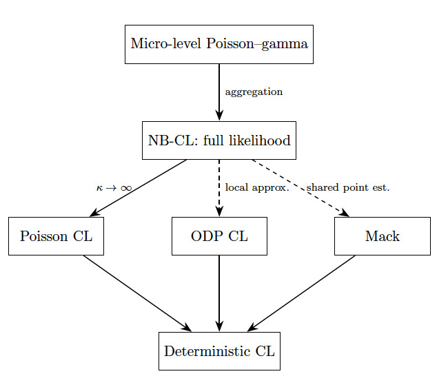
Beyond this micro-level foundation, the NB-CL model provides a unifying probabilistic framework for the entire chain ladder family. The Poisson CL model is an exact special case of the NB-CL likelihood, the ODP model is a locally equivalent quasi-likelihood approximation, and the Mack model is a non-nested specification sharing its point estimates. The residual bootstrap (England and Verrall 2002) is a simulation-based approximation of its predictive distribution. By deriving the CL structure from a micro-level Poisson–gamma process, the NB-CL model clarifies the assumptions underlying classical reserving techniques and places them within a single coherent statistical framework.

1.2. Outline

The remainder of the paper is structured as follows. Section 2 introduces the claims reserving problem and notation. Section 3 presents the NB-CL model. Section 4 derives the model from a micro-level Poisson–gamma construction. Section 5 discusses estimation, including model selection and practical considerations for sparse triangles. Section 6 develops predictive distributions incorporating both process and parameter uncertainty. Section 7 relates the NB-CL model to existing stochastic reserving approaches and presents a model hierarchy. Section 8 presents simulation results under both correct specification and model misspecification. Section 9 provides empirical illustrations on both claim count and paid amount data. Section 10 discusses implications, and Section 11 summarizes our conclusions. Detailed derivations and the accompanying R implementation are collected in Appendices A–C.

2. The claims reserving problem

2.1. Runoff triangles

Non-life insurance claims typically evolve over multiple stages between the occurrence of the underlying event and the final settlement. At each valuation date, the insurer must estimate the outstanding liabilities associated with all claims that have occurred prior to that date.

The standard data structure for macro-level reserving is the runoff triangle. Let \(N_{i,j}\) denote the incremental claim count (or amount) for accident year \(i\) and development year \(j\), where \(i = 1, \ldots, I\) and \(j = 0, \ldots, J-1\). For simplicity, we assume \(I = J\), so the triangle is square. At the valuation date, only the upper-left portion of the triangle is observed, \(\mathcal{D} = \{N_{i,j} : i + j \leq I\}\). The goal is to predict the lower-right portion, \(\mathcal{F} = \{N_{i,j} : i + j > I\}\), and to estimate the total reserve for outstanding counts, \(R^{(N)} = \sum_{i+j > I} N_{i,j}\).

2.2. The deterministic chain ladder method

The classical chain ladder method estimates cumulative development factors from the observed triangle and applies them multiplicatively to project future development. Let \(C_{i,j} = \sum_{l=0}^{j} N_{i,l}\) denote cumulative claims. The development factor for development year \(j\) is \(\hat{f}_j = \sum_{i=1}^{I-j} C_{i,j+1} \big/ \sum_{i=1}^{I-j} C_{i,j}\), for \(j = 0, \ldots, J-2\). The projected ultimate for accident year \(i\) is \(\hat{C}_{i,J-1} = C_{i,I-i} \cdot \prod_{l=I-i}^{J-2} \hat{f}_l\), and the total reserve estimate is \(\hat{R}^{(N)} = \sum_{i=2}^{I} (\hat{C}_{i,J-1} - C_{i,I-i})\).

The deterministic CL method provides point estimates but no measure of uncertainty. The NB-CL model developed in this paper provides a probabilistic foundation that preserves these point estimates exactly in the Poisson limit and approximates them closely for finite \(\kappa\), while enabling coherent uncertainty quantification.

3. The negative binomial–chain ladder model

3.1. Model specification

The NB-CL model assumes that incremental claim counts follow a negative binomial distribution with a log-additive mean structure:

\[ N_{i,j} \sim \text{NegBin}(\mu_{i,j}, \kappa), \quad \log \mu_{i,j} = \alpha_i + \beta_j, \tag{1}\]

where \(\mu_{i,j} = \exp(\alpha_i + \beta_j)\) is the expected count for cell \((i,j)\), \(\alpha_i\) is the accident-year effect, \(\beta_j\) is the development-year effect, and \(\kappa > 0\) is the dispersion parameter controlling overdispersion. We adopt the simplex parameterization \(\sum_{j=0}^{J-1} \exp(\beta_j) = 1\), which gives the development-year effects a direct probabilistic interpretation: \(w_j := \exp(\beta_j)\) is the proportion of ultimate claims reported in development year \(j\), with \(\sum_j w_j = 1\). Under this convention, \(\mu_i := \exp(\alpha_i)\) is the expected total claim count for accident year \(i\), and the cell mean factorizes as \(\mu_{i,j} = \mu_i w_j\).

We use the mean-dispersion parameterization of the negative binomial distribution, under which \(\text{E}[N_{i,j}] = \mu_{i,j}\) and \(\text{Var}(N_{i,j}) = \mu_{i,j} + \mu_{i,j}^2/\kappa\). The variance exceeds the Poisson variance \(\mu_{i,j}\) by a factor that depends on \(\kappa\). As \(\kappa \to \infty\), the variance approaches the Poisson case; as \(\kappa \to 0\), overdispersion becomes extreme.

3.2. Log-additive structure and chain ladder

The log-additive structure \(\log \mu_{i,j} = \alpha_i + \beta_j\) implies \(\mu_{i,j} = \exp(\alpha_i) \cdot \exp(\beta_j)\), a multiplicative decomposition into accident-year and development-year components. This two-way cross-classified structure connects the chain ladder method to the analysis of variance framework (Kremer 1982) and is fundamental to GLM-based reserving.

The ratio of expected cumulative claims between successive development years is

\[\frac{\sum_{l=0}^{j} \mu_{i,l}}{\sum_{l=0}^{j-1} \mu_{i,l}} = \frac{\sum_{l=0}^{j} \exp(\beta_l)}{\sum_{l=0}^{j-1} \exp(\beta_l)},\]

which is constant across accident years. This corresponds exactly to the chain ladder development factor for development year \(j\).

3.3. The dispersion parameter \(\kappa\)

The dispersion parameter \(\kappa\) is best interpreted via the micro-level derivation in Section 4: It represents the variability of cell-level claim-generating conditions around the systematic structure.

Large values of \(\kappa\) (e.g., \(\kappa > 50\)) indicate weak cell-level shocks, with variance close to Poisson. Moderate values (e.g., \(5 < \kappa < 50\)) represent the typical range for many portfolios with meaningful overdispersion. Small values (e.g., \(\kappa < 5\)) indicate strong cell-level shocks (i.e., pronounced departures of individual cells from the multiplicative structure), possibly signaling pattern instability, unmodeled calendar effects, or model misspecification.

4. Micro-level derivation

The NB-CL model is the macro-level aggregation of a Poisson–gamma process with multiplicative development weights.

4.1. Micro-level claim arrival process

Consider a portfolio in which individual claims occur according to a Poisson process. Let \(\lambda_i\) denote the underlying claim arrival rate for accident year \(i\). Conditional on \(\lambda_i\), the number of claims reported in development year \(j\) follows a Poisson distribution:

\[ N_{i,j} \mid \lambda_i \sim \text{Poisson}(\lambda_i w_j), \tag{2}\]

where \(w_j > 0\) is a development weight associated with development year \(j\). These weights capture the reporting pattern and satisfy \(\sum_{j=0}^{J-1} w_j = 1\).

The multiplicative structure of the chain ladder method is recovered by setting \(w_j = \exp(\beta_j)\), which under the simplex constraint \(\sum_j \exp(\beta_j) = 1\) of Section 3 satisfies \(\sum_j w_j = 1\) as required.

Remark 1 (ingredients for the chain ladder estimators). Three assumptions together are sufficient to recover the classical chain ladder development factors from the NB-CL model.

1. Multiplicative mean structure. The log-additive structure \(\log \mu_{i,j} = \alpha_i + \beta_j\) ensures that the ratio of expected cumulative claims between successive development years is constant across accident years, which is the defining property of the chain ladder development factor.

2. Conditional independence across development years. The cell shocks \(\varepsilon_{i,j}\) are independent, so the incremental counts \(N_{i,0}, \ldots, N_{i,J-1}\) are independent, both conditionally and marginally. Without this independence, the column-wise accumulation underlying the development factors would not be well defined.

3. Poisson–gamma hierarchy at the cell level. A gamma shock on the cell rate (Section 4.2) yields the negative binomial marginal and the full likelihood. The multiplicative mean structure alone, or a non-gamma mixing distribution, would give a different marginal distribution and a different likelihood, even if point estimates coincidentally agreed for a particular parameterization. As such, the level at which the shock enters matters as much as its family: A frailty shared by an entire accident year produces the same cell marginals but a different joint law, whose dispersion is not estimable from a single triangle (Remark 2).

The first two ingredients suffice to recover the chain ladder point estimates when estimation proceeds by Poisson or quasi-Poisson scoring, which solves the marginal-totals equations; under the negative binomial likelihood with finite \(\kappa\) the working weights differ from the Poisson weights and the estimates depart slightly from the classical ones (Section 8.2). The third ingredient is required for the full likelihood and the coherent predictive distribution developed in Section 6.

4.2. Gamma shocks at the cell level

Beyond the systematic accident-year and development effects, individual cells depart from the fitted multiplicative structure because the claim-generating environment fluctuates from one (accident-year, development-year) period to the next: short-lived operational, reporting, or exposure conditions local to a cell rather than shared across a row. To capture this residual cell-level variability, we equip each cell with a multiplicative gamma shock:

\[\small{ N_{i,j} \mid \varepsilon_{i,j} \sim \mathrm{Poisson}\!\big(\exp(\alpha_i)\, w_j\, \varepsilon_{i,j}\big), \qquad \varepsilon_{i,j} \sim \mathrm{Gamma}(\kappa, \kappa) \ \text{i.i.d.}, \tag{3}}\]

with \(\mathrm{E}[\varepsilon_{i,j}] = 1\) and \(\mathrm{Var}(\varepsilon_{i,j}) = 1/\kappa\). Marginalizing over the shock yields \(N_{i,j} \sim \mathrm{NegBin}(\mu_{i,j}, \kappa)\) with \(\mu_{i,j} = \exp(\alpha_i) w_j\), independently across cells, which is exactly the likelihood (5) maximized in Section 5.

The gamma distribution is a natural choice for modeling heterogeneity in Poisson rates, both because it is conjugate to the Poisson and because it leads to a closed-form marginal distribution. This Poisson–gamma structure has deep connections to credibility theory (Bühlmann and Straub 1970), where gamma-distributed random effects capture heterogeneity across risk classes. Gisler and Wüthrich (2008) develop this connection specifically for claims reserving, showing that Bühlmann–Straub credibility estimators provide a natural interpretation of chain ladder development factors and yield refined uncertainty estimates by combining individual accident-year information with portfolio-level pooling. A credibility reading of the chain ladder family requires a hierarchical level structure, with accident-year levels drawn around a common center or anchored by exposure, so that information pools across rows. The NB-CL model as specified here, with a free \(\alpha_i\) per accident year, deliberately performs no such pooling: Each row’s level is estimated from that row alone, and the gamma layer of equation (3) operates at the cell level. The likelihood-based credibility counterpart of Gisler and Wüthrich (2008) hence only requires a common-rate, exposure-anchored hierarchy on the levels, and is developed in Van Oirbeek (2026).

Proposition 1 (conjugacy of the gamma shock). Among unit-mean mixing distributions on \((0,\infty)\), the gamma family is the conjugate family for Poisson sampling (Diaconis and Ylvisaker 1979). Conjugacy closes the mixing integral in negative binomial form, places the marginal in the exponential dispersion family (thereby enabling profile-likelihood estimation of \(\kappa\) within a standard GLM), and yields the linear posterior mean underlying credibility formulas (Jewell 1974).

Non-conjugate mixing distributions lose the GLM machinery, not identifiability. The lognormal mixture has no closed-form marginal; the inverse Gaussian has a closed-form marginal (Willmot 1987) that lies outside the exponential dispersion family, so \(\kappa\) is then estimated by direct numerical likelihood rather than via glm.nb. Note that the inverse Gaussian belongs to the natural exponential family with power variance function (Tweedie power \(p = 3\)): The tractability of the gamma choice is a consequence of Poisson conjugacy specifically, not of NEF-PVF membership.

4.3. Marginal distribution of incremental counts

Marginalizing over the cell-level shock \(\varepsilon_{i,j}\) is the well-known Poisson–gamma mixture, which yields a negative binomial distribution for the incremental counts:

\[ N_{i,j} \sim \text{NegBin}(\mu_{i,j}, \kappa), \quad \mu_{i,j} = \exp(\alpha_i) \cdot w_j. \tag{4}\]

Taking logarithms and absorbing the normalization into \(\beta_j\) gives \(\log \mu_{i,j} = \alpha_i + \beta_j\), which recovers the NB-CL model specification (1). The mixing integral and a full proof are given in Appendix A.

Proposition 2 (Poisson–gamma mixture). Let \(N \mid \lambda \sim \text{Poisson}(\lambda w)\) and \(\lambda \sim \text{Gamma}(\kappa, \kappa/\mu)\). Then \(N \sim \text{NegBin}(\mu w, \kappa)\) with \(\text{E}[N] = \mu w\) and \(\text{Var}(N) = \mu w + (\mu w)^2/\kappa\).

Note that the cumulative counts inherit the conditional-Poisson structure: Conditional on the shocks, the cumulative count \(C_{i,j} = \sum_{l \leq j} N_{i,l}\) is again Poisson, and the constancy of the expected age-to-age factors across accident years—the defining chain ladder property—is a property of the marginal mean that emerges once the unit-mean shocks are averaged out. The CL formula is therefore not an algebraic coincidence but follows from the conditional-Poisson cell structure together with the unit-mean normalization of the shocks; the formal statement is given in Appendix A.

4.4. Interpretation of \(\kappa\)

The dispersion parameter \(\kappa\) controls the variability of cell-level conditions around the systematic multiplicative structure. As \(\kappa \to \infty\) the shocks degenerate and the model reduces to the Poisson chain ladder; for finite \(\kappa\), \(\mathrm{Var}(N_{i,j}) = \mu_{i,j} + \mu_{i,j}^2/\kappa\), which exceeds the Poisson variance and reflects overdispersion due to cell-level shocks.

Remark 2 (accident-year frailty is absorbed by the \(\alpha_i\)). Replacing the cell-level shocks in equation (3) by a single frailty shared across an accident year (i.e., \(\lambda_i \sim \mathrm{Gamma}(\kappa, \kappa/\exp(\alpha_i))\)) with cells conditionally independent given \(\lambda_i\), produces the same negative binomial marginals but a different joint law, whose likelihood factorizes into a negative binomial row total and a frailty-free multinomial split. With free \(\alpha_i\) the realized frailty is absorbed into the fitted accident-year parameter, and the frailty dispersion is not identifiable from a single triangle. The reason is visible in the factorization: The multinomial split carries no frailty, since a row-level frailty scales all cells of a row equally and cancels in the conditional split, while the negative binomial row-total component is fitted exactly by the free \(\alpha_i\), leaving a profile likelihood that increases monotonically in \(\kappa\) toward the Poisson limit. Numerically, fitting equation (5) to data generated from the year-level model with \(\kappa = 10\) returns \(\hat{\kappa}\) in the hundreds of thousands or larger in every replication. The dispersion the NB-CL model estimates is therefore the cell-level \(\kappa\) of equation (3); accident-year heterogeneity is identified only through anchored or hierarchical levels and is outside the scope of the present model.

4.5. The \(\kappa \to 0\) limit

The limit \(\kappa \to 0\) represents extreme cell-level shock dispersion. In this regime, the gamma shocks \(\varepsilon_{i,j} \sim \mathrm{gamma}(\kappa,\kappa)\) of equation (3) become increasingly diffuse: \(\mathrm{Var}(\varepsilon_{i,j}) = 1/\kappa \to \infty\), so individual cells depart arbitrarily far from the multiplicative structure. The cell-level variance explodes accordingly, \(\mathrm{Var}(N_{i,j}) \approx \mu_{i,j}^2/\kappa \to \infty\).

The practical implication for reserving is that age-to-age factors become unreliable. A development factor \(\hat{f}_j\) is a ratio of cumulative counts across accident years. When the counts in any row have near-infinite variance, the numerator and denominator of this ratio are both highly unstable, and the resulting factor can take extreme values. Reserve estimates for individual accident years may diverge widely as a consequence, even if the total reserve remains finite in expectation.

No borrowing of strength across rows occurs in this model at any value of \(\kappa\): with a free \(\alpha_i\) per accident year, each row’s level is estimated from that row alone. Cross-row pooling, i.e., the credibility-theoretic content of the Poisson–gamma hierarchy (Bühlmann and Straub 1970), requires a hierarchical structure on the levels and is developed in Van Oirbeek (2026).

The profile likelihood for \(\kappa\) also flattens as \(\kappa \to 0\), making estimation unstable in this regime.

Remark 3 (multinomial split given the row total). The conditional-Poisson cell structure (Appendix A) implies a multinomial development split. Conditional on the shock vector \((\varepsilon_{i,0},\ldots,\varepsilon_{i,J-1})\) and on the row total \(N_i = \sum_j N_{i,j}\), the vector of increments is multinomial with cell probabilities proportional to \(w_j \varepsilon_{i,j}\). In the Poisson limit \(\kappa \to \infty\) the shocks degenerate and the split reduces to \(\mathrm{Multinomial}(N_i, \pmb{w})\): Each claim is allocated independently to development period \(j\) with probability \(w_j\). This is the point of contact with multinomial development models such as the Dirichlet–multinomial framework of Sriram and Shi (2021) (Section 7.5), which places the variability on the split probabilities themselves rather than on cell-level rates.

5. Estimation

5.1. Log-likelihood

Under the NB-CL model, the log-likelihood for the observed triangle is

\[ \ell(\pmb{\alpha}, \pmb{\beta}, \kappa) = \sum_{i=1}^{I} \sum_{j=0}^{I-i} \log f_{\text{NegBin}}(N_{i,j}; \mu_{i,j}, \kappa), \tag{5}\]

where \(f_{\text{NegBin}}\) denotes the negative binomial probability mass function in the mean-dispersion parameterization; its explicit log-density is recalled in Appendix A.

5.2. Identifiability constraints

The log-additive structure \(\log \mu_{i,j} = \alpha_i + \beta_j\) is not identifiable without constraints, since adding a constant to all \(\alpha_i\) and subtracting the same constant from all \(\beta_j\) leaves \(\mu_{i,j}\) unchanged. We impose the simplex constraint \(\sum_{j=0}^{J-1} \exp(\beta_j) = 1\) of Section 3, which gives \(w_j = \exp(\beta_j)\) the interpretation of a development-pattern probability and makes \(\mu_i = \exp(\alpha_i)\) the expected total claim count for accident year \(i\).

Standard GLM software (e.g., MASS::glm.nb) imposes identifiability via the treatment-contrast convention \(\tilde{\beta}_0 = 0\) instead, returning coefficients \((\tilde{\alpha}_i, \tilde{\beta}_j)\) that do not satisfy the simplex constraint. The post hoc transformation to the simplex-parameterized coefficients used throughout this paper is a one-to-one reparameterization that leaves the cell means \(\mu_{i,j}\), the likelihood, the dispersion estimate \(\hat{\kappa}\), and all predictive quantities unchanged; only the interpretation of the individual \(\alpha_i\) and \(\beta_j\) coefficients shifts. The transformation is given in Appendix C.

5.3. Estimation via GLM

The NB-CL model is a GLM with negative binomial response and log link. Estimation proceeds in two stages. First, for fixed \(\kappa\), the conditional MLEs of \((\pmb{\alpha}, \pmb{\beta})\) are obtained by fitting a GLM with negative binomial family and log link. Second, the dispersion parameter \(\kappa\) is estimated by maximizing the profile likelihood \(\ell_p(\kappa) = \ell(\hat{\pmb{\alpha}}(\kappa), \hat{\pmb{\beta}}(\kappa), \kappa)\).

In R, this can be implemented using MASS::glm.nb, which performs both steps automatically.

5.4. Connection to classical chain ladder estimators

In the limit \(\kappa \to \infty\), the negative binomial distribution reduces to the Poisson, and the NB-CL model becomes a Poisson GLM with log link. In this case, the MLEs of \(\alpha_i\) and \(\beta_j\) coincide with the classical chain ladder estimators, the fitted values \(\hat{\mu}_{i,j}\) reproduce the chain ladder projections, and the variance reduces to \(\text{Var}(N_{i,j}) = \mu_{i,j}\).

Thus, the NB-CL model generalizes the classical chain ladder method while preserving its point estimates in the Poisson limit.

5.5. Model selection: Testing for overdispersion

Since the Poisson CL model is nested within the NB-CL model as the limiting case \(\kappa \to \infty\), formal model selection tools can be applied to assess whether the additional dispersion parameter is warranted.

Likelihood ratio test.

The null hypothesis \(H_0: \kappa = \infty\) (Poisson) can be tested against \(H_1: \kappa < \infty\) (NB-CL) via the likelihood ratio statistic \(\Lambda = 2\bigl[\ell_{\text{NB}}(\hat{\pmb{\alpha}}, \hat{\pmb{\beta}}, \hat{\kappa}) - \ell_{\text{Pois}}(\hat{\pmb{\alpha}}_0, \hat{\pmb{\beta}}_0)\bigr]\), where \(\ell_{\text{NB}}\) and \(\ell_{\text{Pois}}\) denote the maximized log-likelihoods of the NB-CL and Poisson CL models, respectively. Under \(H_0\), the parameter \(\kappa\) lies on the boundary of the parameter space, so the standard \(\chi^2_1\) reference distribution does not apply. Instead, \(\Lambda\) follows a 50:50 mixture of a point mass at zero and \(\chi^2_1\) (Self and Liang 1987), yielding a \(p\)-value of \(\frac{1}{2}\Pr(\chi^2_1 \geq \Lambda)\).

In both empirical illustrations (Section 9), the test is decisive. For the Australian motor bodily injury count data, \(\Lambda = 2{,}550.1\) (\(p < 10^{-20}\)); for the Taylor–Ashe paid amounts data, \(\Lambda = 1{,}902{,}378\) (\(p < 10^{-20}\)).

Information criteria.

\(\text{AIC} = -2\ell + 2p\) and \(\text{BIC} = -2\ell + p \log n\) provide complementary model selection tools that do not require boundary corrections, where \(p\) is the number of parameters (the NB-CL model has one additional parameter relative to the Poisson CL). For the Australian count data, \(\Delta\text{AIC} = 2{,}548\) in favor of the NB-CL model; for the Taylor–Ashe data, \(\Delta\text{AIC} = 1{,}902{,}376\). When \(\Delta\text{AIC}\) or \(\Delta\text{BIC}\) is close to zero, the simpler Poisson CL model may be preferred on parsimony grounds.

5.6. Practical considerations

5.6.1. Zero and sparse cells

Real triangles often contain zeros, especially in the tail (late development years, recent accident years). For Poisson and negative binomial GLMs with log link, zero cells are permissible since the negative binomial assigns positive probability to zero. If, however, an entire row or column is zero, separation occurs and the MLE for that \(\alpha_i\) or \(\beta_j\) diverges to \(-\infty\). Even near-zero cells can cause near-separation and inflated standard errors.

5.6.2. Small triangles

For small triangles (e.g., \(I = 5\) or \(6\)), the number of parameters approaches the number of observations. With \(I\) accident-year effects, \(I - 1\) development-year effects (one constrained), and one dispersion parameter, we have approximately \(2I\) parameters from \(I(I+1)/2\) cells. Overfitting is a real risk.

For sparse triangles, practitioners should consider parsimonious models with parametric development curves (reducing the number of \(\beta_j\) parameters), hierarchical models that shrink \(\alpha_i\) toward a common mean, or ridge regularization by adding a penalty \(\lambda(\sum_i \alpha_i^2 + \sum_j \beta_j^2)\) to the log-likelihood.

5.6.3. Diagnostics

We recommend examining the profile likelihood for \(\kappa\) to verify that it is unimodal and well peaked rather than flat or multimodal. The standard errors on \(\alpha_i\) should be stable; if they explode for recent accident years, this indicates estimation problems. Pearson residuals should be consistent with negative binomial assumptions, showing no systematic patterns across accident years, development years, or calendar years. Finally, the condition number of the Hessian should be monitored, with values above 1,000 suggesting numerical instability.

5.6.4. Interpreting extreme values of \(\hat{\kappa}\)

The dispersion parameter \(\kappa\) governs the degree of cell-level overdispersion—the variability of individual cells around the fitted multiplicative structure—with smaller values indicating greater overdispersion. Table 1 provides guidance for interpretation.

At \(\kappa = 1\), the negative binomial reduces to the geometric distribution, implying that the coefficient of variation of the cell-level shocks is 100%—individual cells depart strongly from the multiplicative structure.

Remark 4 (warning signs for small \(\hat{\kappa}\)). In practice, estimates of \(\hat{\kappa} < 3\) are rare and should prompt investigation rather than blind application of the model. Such extreme heterogeneity may indicate structural breaks in the portfolio (such as mergers, product changes, or underwriting shifts), unmodeled calendar-year effects that have been absorbed into the dispersion parameter, or data quality issues and coding errors. The simulation study in Section 8 demonstrates that the NB-CL model with bias-corrected \(\kappa\) maintains good coverage even at \(\kappa = 2\), so the method remains reliable in these extreme cases. Nevertheless, practitioners encountering \(\hat{\kappa} < 3\) should examine residual diagnostics, test for calendar-year effects, and consider whether the log-additive structure is appropriate for the portfolio.

6. Predictive distribution and uncertainty quantification

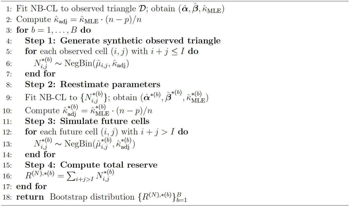
The NB-CL likelihood yields a coherent predictive distribution for future incremental claims and for the total reserve. The plug-in form accounts for process variance only; parameter uncertainty is added via the parametric bootstrap of Section 6.4.

6.1. Plug-in predictive distribution

Conditional on the estimated parameters \((\hat{\pmb{\alpha}}, \hat{\pmb{\beta}}, \hat{\kappa})\), the future incremental counts satisfy

\[ N_{i,j}^{\text{future}} \sim \text{NegBin}(\hat{\mu}_{i,j}, \hat{\kappa}), \quad i + j > I, \tag{6}\]

where \(\hat{\mu}_{i,j} = \exp(\hat{\alpha}_i + \hat{\beta}_j)\). The total reserve is \(R^{(N)} = \sum_{i+j > I} N_{i,j}^{\text{future}}\). Since future cells are conditionally independent given the parameters, the distribution of \(R^{(N)}\) can be computed via convolution or Monte Carlo simulation.

6.2. Process variance only

The plug-in predictive distribution equation (6) incorporates process variance (i.e., the inherent randomness in future claim counts given fixed, known parameters). Hence, it quantifies how much future counts would vary around their mean if the true parameter vector \(\pmb{\theta} = (\pmb{\alpha}, \pmb{\beta}, \kappa)\) were known exactly.

The parameters, however, are not known. They are estimated from the same observed triangle \(\mathcal{D}\) that is used to make the predictions. A different realization of the triangle would yield different estimates \((\hat{\pmb{\alpha}}, \hat{\pmb{\beta}}, \hat{\kappa})\) and therefore different predicted reserves. This additional variability (i.e., the extent to which the reserve estimate changes as a function of which triangle was observed) is estimation variance, and it is ignored by the plug-in approach.

The decomposition

\[ \mathrm{Var}(R) = \underbrace{\mathrm{E}[\mathrm{Var}(R \mid \pmb{\theta})]}_{\text{process variance}} + \underbrace{\mathrm{Var}(\mathrm{E}[R \mid \pmb{\theta}])}_{\text{estimation variance}} \tag{7}\]

formalizes this distinction. The plug-in distribution accounts only for the first term. For typical triangle sizes, estimation variance is of the same order as process variance and cannot be neglected. Predictive intervals based solely on process variance will therefore undercover systematically: The true outstanding counts will fall outside the nominal interval more often than the stated level implies. The parametric bootstrap developed in Section 6.4 accounts for both terms simultaneously.

6.3. Variance decomposition

The total predictive variance decomposes as shown in equation (7), mirroring the structure of Mack (1993) but arising here from a fully specified likelihood model rather than second-moment assumptions alone.

6.4. Parametric bootstrap

To incorporate both process and estimation variance, we employ a parametric bootstrap procedure.

6.4.1. Adjusted profile likelihood and bias correction

Maximum likelihood estimation of \(\kappa\) via the profile likelihood \(\ell_p(\kappa)\) is subject to finite-sample bias. The profile likelihood treats the estimated means \(\hat{\pmb{\mu}}(\kappa)\) as though they were known, ignoring the information consumed in estimating the \(p\)-dimensional nuisance parameter \(\pmb{\lambda} = (\pmb{\alpha}, \pmb{\beta})\). For runoff triangles where \(n = I(I+1)/2\) is modest relative to \(p \approx 2I - 1\), this bias can be substantial. Empirically, \(\hat{\kappa}_{\text{MLE}}\) tends to overestimate the true \(\kappa\), leading to underestimation of variance and hence undercoverage of predictive intervals.

The appropriate correction is the Cox–Reid adjusted profile likelihood (Cox and Reid 1987; Barndorff-Nielsen 1983), which penalizes the profile likelihood by half the log-determinant of the observed information matrix for the nuisance parameters, thereby removing the \(O(1)\) bias in \(\ell_p(\kappa)\) that arises from nuisance parameter estimation. Evaluating this adjustment for the NB-CL likelihood under the approximation that the design is balanced and that fitted means are not negligible relative to \(\kappa\) yields a correction to the profile score of order \(p/(2\kappa)\); the derivation, together with a discussion of the scope of the approximation, is given in Appendix B. Solving, the leading-order adjustment to the MLE is

\[ \hat{\kappa}_{\mathrm{adj}} = \hat{\kappa}_{\mathrm{MLE}} \cdot \frac{n - p}{n}. \tag{8}\]

In the Poisson limit \(\kappa \to \infty\), the NB variance function reduces to \(v = \mu\), the profile score equation for \(\kappa^{-1}\) becomes linear, and the correction factor \((n-p)/n\) is exact, coinciding with the restricted maximum likelihood correction for Gaussian variance components (Patterson and Thompson 1971) and with the degrees-of-freedom correction for the quasi-Poisson dispersion parameter (McCullagh and Nelder 1989). The correction is therefore not novel in itself; what is novel is its derivation as a Cox–Reid adjustment specific to the NB-CL likelihood.

For a \(10 \times 10\) triangle, \(n = 55\) and \(p = 19\) (one intercept, nine accident-year effects, nine development-year effects), the correction factor is approximately 0.65. Here \(p\) counts only the mean (nuisance) parameters \(\pmb{\lambda}\); the interest parameter \(\kappa\) is excluded from the Cox–Reid adjustment. The parameter count of Section 5.5, which includes \(\kappa\), serves the different purpose of overfitting assessment. This correction shrinks \(\hat{\kappa}\) toward smaller values, appropriately increasing the estimated variance. The simulation study in Section 8 demonstrates that this correction yields well-calibrated predictive intervals across a wide range of \(\kappa\) values.

6.4.2. Bootstrap algorithm

Algorithm 1.Parametric bootstrap for NB-CL with bias-corrected \(\kappa\).

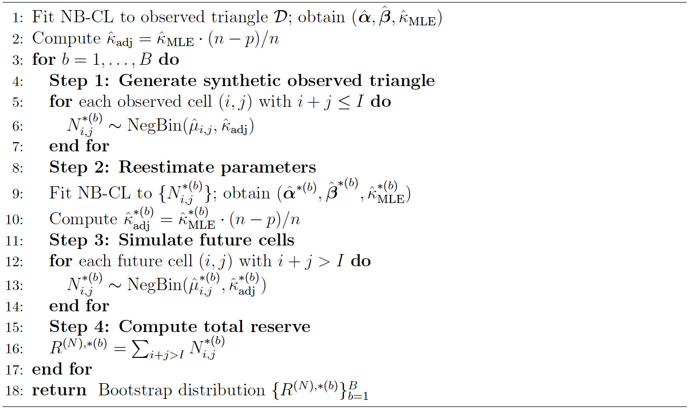
Predictive intervals are obtained as empirical quantiles of the bootstrap distribution. For example, the 95% predictive interval is \([R^{(N), *(0.025)}, R^{(N), *(0.975)}]\).

Remark 5 (Bootstrap design and parameter uncertainty). Algorithm 1 propagates estimation uncertainty in \((\pmb{\alpha}, \pmb{\beta}, \kappa)\) by reestimating all parameters on each synthetic triangle, following the standard parametric bootstrap for predictive intervals (Davison and Hinkley 1997). This approach treats the observed triangle as one realization of the fitted model and asks how much reserve estimates would vary across realizations, capturing both process variance and parameter estimation variance simultaneously. A theoretically distinct procedure places explicit priors on \((\pmb{\alpha}, \pmb{\beta}, \kappa)\) and integrates the predictive distribution against the resulting posterior; this Bayesian alternative is discussed in Section 10.4 and is the recommended approach for small triangles where the quadratic approximation underlying the bias correction is least accurate.

6.5. Comparison with the residual (ODP) bootstrap

The parametric bootstrap described above differs from the residual bootstrap of England and Verrall (2002) in several ways. It does not rely on the ODP quasi-Poisson variance structure and does not resample Pearson residuals. Instead, it resamples from a fully specified negative binomial distribution and naturally extends to any distributional assumption, such as Tweedie for amounts.

Despite these differences, both approaches share the goal of quantifying process and estimation variance. The NB-CL bootstrap achieves this with fewer assumptions and a clearer probabilistic interpretation. A further practical advantage is that tail quantiles of the reserve distribution, such as the 1-in-100 or 1-in-500 outcome relevant for capital setting, are estimated by sampling from a fully specified parametric family rather than from a finite pool of residuals. For a \(10 \times 10\) triangle the residual pool contains only 55 observations, making extreme-quantile estimates from residual resampling unreliable; the parametric bootstrap does not share this limitation.

7. Relationship to existing models

The NB-CL model provides a unifying framework that encompasses several well-known stochastic extensions of the chain ladder method, though the nature of the relationship differs across models.

7.1. Poisson chain ladder

The Poisson chain ladder model assumes \(N_{i,j} \sim \text{Poisson}(\mu_{i,j})\) with \(\log \mu_{i,j} = \alpha_i + \beta_j\). This is a special case of the NB-CL model obtained by letting \(\kappa \to \infty\). In this limit, \(\text{Var}(N_{i,j}) = \mu_{i,j}\), and the negative binomial reduces to the Poisson.

7.2. Overdispersed Poisson chain ladder

The ODP model assumes \(\operatorname{Var}(N_{i,j}) = \phi\, \mu_{i,j}\), where \(\phi > 1\) is an overdispersion parameter. This variance structure is motivated by quasi-likelihood theory rather than a fully specified probability distribution.

The relationship between the ODP model and Mack’s distribution-free chain ladder (DFCL) model has been the subject of extended methodological debate. Mack and Venter (2000) provide a detailed comparison and show that, although both models reproduce the chain ladder point estimates, they differ structurally in their independence assumptions, in the fitted values they imply within the observed triangle, and in their behavior when the data structure deviates from a strict triangle (e.g., trapezoidal data, missing cells, or alternative weighting of development factors). They conclude that only the DFCL model qualifies as the stochastic model underlying the chain ladder algorithm. The NB-CL model offers a third route that is not subject to their critique: Rather than selecting between two ad hoc working models on the basis of which are considered closer to the deterministic algorithm, it derives the chain ladder structure from a coherent micro-level process. The DFCL/ODP debate becomes a question of which approximation to the NB-CL likelihood is preferred, not which model truly underlies the algorithm.

The technical content of this resolution lies in the variance functions. The NB2 parameterization adopted here implies a quadratic variance-mean relationship, \(\operatorname{Var}(N_{i,j}) = \mu_{i,j} + \mu_{i,j}^2/\kappa\), whereas the ODP model assumes a linear relationship \(\operatorname{Var}(N_{i,j}) = \phi\,\mu_{i,j}\). These two variance profiles are structurally distinct: The ODP variance function is not a special case of the NB2 variance function for any value of \(\kappa\). The connection between them is nonetheless precise. Rewriting the NB2 variance as \(\mu_{i,j}\bigl(1 + \mu_{i,j}/\kappa\bigr)\) shows that, if cell means are approximately equal to some portfolio average \(\bar{\mu}\), the NB2 variance coincides with the ODP variance under the identification \(\phi = 1 + \bar{\mu}/\kappa\). This is a local approximation valid when the range of \(\mu_{i,j}\) across cells is narrow relative to \(\kappa\); it breaks down in cells with large counts where the quadratic term dominates.

The ODP model can also be embedded in a proper likelihood framework through the NB1 parameterization, under which \(\operatorname{Var}(N_{i,j}) = \mu_{i,j}(1+\psi)\) for some \(\psi > 0\), yielding a linear variance-mean relationship that exactly matches ODP. The NB2 formulation adopted in the present paper implies a quadratic relationship instead, which is more appropriate when overdispersion increases with the magnitude of expected counts, a pattern commonly observed in cells with large exposure. The choice between NB1 and NB2 is an empirical question assessable via residual diagnostics or likelihood-based model comparison.

7.3. Negative-binomial model of Verrall

A closely related but structurally distinct negative binomial model was proposed by Verrall (2000) and is presented in Wüthrich and Merz (2008) as a conditional time-series formulation. That model specifies:

\[X_{i,j} \mid C_{i,j-1} \;\sim\; \mathrm{NB1}\!\left(C_{i,j-1}(f_{j-1}-1),\; f_{j-1}\right), \tag{9}\]

where \(\mathrm{NB1}(m, \delta)\) denotes a negative binomial distribution parameterized by its mean \(m\) and its variance-to-mean ratio \(\delta\), so that the variance is linear in the mean. This is deliberately distinct from the mean-dispersion (NB2) convention \(\mathrm{NegBin}(\mu, \kappa)\) used throughout this paper, under which the variance is quadratic in the mean; the Verrall model cannot be written in the NB2 notation. Its conditional mean is \(C_{i,j-1}(f_{j-1}-1)\) and its conditional variance \(C_{i,j-1}(f_{j-1}-1)f_{j-1}\). This differs from the NB-CL model in two structural respects.

First, the dispersion parameter in equation (9) is \(f_{j-1}\), which varies by development year. The NB-CL model has a single constant dispersion parameter \(\kappa\) across all cells, reflecting the assumption of a homogeneous cell-level shock distribution, where \(\kappa\) is a property of the residual claim-generating environment, not of the development pattern. The Verrall (2000) model is not without a derivation: It arises as the negative binomial recursion obtained when the row parameters of the cross-classified (overdispersed) Poisson model are integrated against a gamma prior, as presented in Wüthrich and Merz (2008). What it does not supply is a micro-level account of why the dispersion should equal the development factor, since the recursion delivers that identity as an algebraic consequence of the conditioning rather than as a property of the claim-generating process. It is, in the terminology of Section 7.2, an NB1-type specification with a development-year–specific variance-to-mean ratio.

Second, the Verrall (2000) model is formulated conditionally on the cumulative \(C_{i,j-1}\), making it a time-series model in the spirit of the Mack assumptions. The NB-CL model is formulated unconditionally at the cell level, with the multiplicative mean structure \(\log\mu_{i,j} = \alpha_i + \beta_j\) arising from the Poisson–gamma micro-derivation rather than from recursive development.

Both models are consistent with the chain ladder assumptions (Mack 1993). The Verrall (2000) model reproduces the chain ladder point estimates; the NB-CL estimates coincide with them in the Poisson limit and approximate them closely for finite \(\kappa\) (Section 8.2). The models further differ in their variance functions, in the interpretation of the dispersion parameter, and in whether the dispersion is constant or development-varying. The NB-CL model is preferable when the goal is a structural interpretation of overdispersion as cell-level shock variability; the Verrall (2000) model may be preferable when the development pattern itself is believed to drive the overdispersion.

7.4. Mack model

The Mack model (Mack 1993) is formulated conditionally on cumulative claims: \(\mathbb{E}[C_{i,j+1} \mid C_{i,j}] = f_j\, C_{i,j}\) and \(\mathrm{Var}(C_{i,j+1} \mid C_{i,j}) = \sigma_j^2\, C_{i,j}\), with independence across accident years. It specifies only these conditional first and second moments, assumes no full probability distribution, and obtains the mean squared error of prediction analytically rather than by resampling.

The NB-CL model differs in three respects. First, it specifies a full likelihood rather than conditional moments. Second, its second-moment structure is unconditional, constant dispersion, and quadratic in the cell mean, whereas Mack’s is conditional, column specific, and linear in the cumulative; the two specifications are non-nested, as Mack and Venter (2000) emphasize in the parallel ODP/DFCL comparison. Third, prediction uncertainty in the NB-CL model follows from the predictive distribution itself (Section 6), not from separate variance formulas.

The Mack model is therefore not a moment truncation of the NB-CL model; it is an alternative, non-nested second-moment specification that shares the chain ladder point estimates.

7.5. Dirichlet–multinomial chain ladder

The Dirichlet–multinomial chain ladder model places a Dirichlet prior on the multinomial probabilities governing the development pattern, with a concentration parameter \(c\) controlling the variability of the development pattern across accident years. Sriram and Shi (2021) develop this framework to unify the chain ladder and Bornhuetter–Ferguson methods within a single Bayesian model: CL emerges when conditioning on observed row totals, while BF emerges when integrating out the ultimates under a strong prior. Marginalizing over the Dirichlet prior yields a negative binomial distribution for aggregated counts, paralleling the Poisson–gamma route taken in this paper.

The NB-CL model and the Dirichlet–multinomial framework capture different sources of heterogeneity and are therefore complementary rather than equivalent. The NB-CL dispersion parameter \(\kappa\) captures cell-level shock variability around the multiplicative structure (arrival-rate heterogeneity across accident years being absorbed by the free \(\alpha_i\); Remark 2). The Dirichlet concentration parameter \(c\) captures variability in the development pattern itself across accident years, holding the arrival rate fixed. Both lead to negative binomial marginals for incremental counts but the underlying generative mechanisms are distinct, and a model that incorporates both layers simultaneously would extend the present framework. The NB-CL model is formulated directly at the incremental level and is naturally expressed as a GLM with log link, which facilitates standard estimation; the Dirichlet–multinomial formulation is more naturally Bayesian.

7.6. Hierarchical Bayesian chain ladder

Taylor (2015) surveys Bayesian formulations of the chain ladder method within a unifying framework in which error terms belong to the exponential dispersion family, with overdispersed Poisson and Tweedie errors arising as special cases; both the Mack and the cross-classified forms are treated, with priors on row, column, or diagonal parameters and estimation via MCMC.

The NB-CL model and Taylor’s framework are complementary rather than competing, since both embed the chain ladder within a probabilistic hierarchy that accommodates accident-year heterogeneity. They differ in three respects: the NB-CL model is derived from a micro-level Poisson–gamma construction (Section 4) that gives the dispersion parameter \(\kappa\) a structural interpretation as the inverse variance of the cell-level shocks, whereas Taylor’s framework specifies the hierarchy directly at the macro level; the NB-CL model admits estimation via standard GLM software (MASS::glm.nb in R), requiring no MCMC implementation and converging in seconds even for large triangles; and the NB-CL model preserves the classical chain ladder point estimates exactly in the Poisson limit \(\kappa \to \infty\), thereby providing a clean nesting structure that connects the stochastic and deterministic versions of the method. The Bayesian approach of Taylor (2015) is preferable when prior information is available or when the triangle is too sparse for reliable maximum likelihood estimation. The NB-CL model is better suited as a default frequentist framework, and Section 10.4 sketches the natural Bayesian extension.

7.7. Model hierarchy

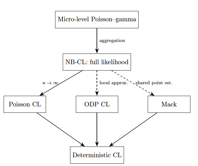
Figure 1 illustrates the relationships among chain ladder reserving models. The NB-CL model is directly linked to micro-level Poisson–gamma processes, induces a negative binomial distribution at the macro level, and admits a GLM formulation. The Poisson CL model is an exact special case (\(\kappa \to \infty\)). The Mack model is a non-nested second-moment specification that shares the chain ladder point estimates but conditions on cumulatives with column-specific variance parameters (Section 7.4). The ODP CL model is structurally distinct from NB-CL in its variance function but shares the same mean structure, with point estimates coinciding in the Poisson limit. The dashed arrow in Figure 1 denotes a local approximation between the two variance functions, valid when cell means are approximately homogeneous (Section 7.2).

Figure 1.Relationships among chain ladder reserving models. Solid arrows denote exact special cases; dashed arrows denote non-nested relationships. The latter encompass two scenarios: a local approximation between the NB2 and ODP variance functions under approximately homogeneous cell means, and the Mack case, which features shared point estimates but structurally different, conditional second moments. Neither ODP CL nor the Mack model is a special case of NB-CL. See Sections 7.2 and 7.4 for details.

8. Simulation study

Three questions are addressed by simulation: the size of the bias correction for \(\kappa\) developed in Section 6.4.1, the calibration of NB-CL predictive intervals against Poisson CL and ODP CL under correct specification, and the robustness of the method under three forms of misspecification.

8.1. Simulation design

We generate synthetic runoff triangles directly from the NB-CL model to evaluate coverage properties under correct specification.

8.1.1. Data-generating process

For each cell \((i,j)\) in the triangle, counts are generated from the NB-CL model (1) with true parameters \((\alpha_i^{\mathrm{true}}, \beta_j^{\mathrm{true}}, \kappa^{\mathrm{true}})\), i.e., \(N_{i,j} \sim \operatorname{NegBin}(\mu_{i,j}, \kappa^{\mathrm{true}})\) with \(\log \mu_{i,j} = \alpha_i^{\mathrm{true}} + \beta_j^{\mathrm{true}}\). The observed triangle consists of cells with \(i + j \leq I\); the remaining cells constitute the future development, and the true outstanding counts are \(R_{\cdot}^{(N),\mathrm{true}} = \sum_{i+j > I} N_{i,j}\).

8.1.2. Parameter settings

Triangles of size \(I = J = 10\) are generated, yielding 55 observed cells and 45 future cells. Accident-year effects are set as \(\alpha_i^{\mathrm{true}} = \log\bigl(1000 + 500\,(i-1)/9\bigr)\), representing gradual exposure growth across accident years. The development pattern is \((w_0, \ldots, w_9) \propto (0.53, 0.24, 0.12, 0.05, 0.03, 0.015, 0.005, 0.003\), \(0.001, 0.001)\), normalized to sum to one; development effects are \(\beta_j^{\mathrm{true}} = \log w_j - \log w_0\) so that \(\beta_0^{\mathrm{true}} = 0\). For the \(I = 7\) triangles of Panel A the pattern is \((w_0, \ldots, w_6) \propto (0.53, 0.24, 0.12, 0.05, 0.03, 0.02, 0.01)\) with \(\alpha_i^{\mathrm{true}} = \log\!\bigl(1000 + 500(i-1)/6\bigr)\), the remaining settings as above. The dispersion parameter takes values \(\kappa^{\mathrm{true}} \in \{2,\, 3,\, 5,\, 10,\, 20,\, 50\}\), spanning extreme to mild overdispersion. For each setting, \(n_{\mathrm{sim}} = 500\) replications are performed, with \(B = 500\) bootstrap samples per replication.

8.1.3. Methods compared

We compare four methods that share the same chain ladder predictor structure but differ in their distributional assumptions. Poisson CL fits a GLM with Poisson family and therefore ignores any overdispersion present in the data. ODP CL fits a GLM with quasi-Poisson family, estimating the overdispersion parameter \(\phi\) from the Pearson residuals; this is the standard approach underlying the ODP bootstrap of England and Verrall (2002). NB-CL (MLE) fits a GLM with negative binomial family and uses the maximum likelihood estimate \(\hat{\kappa}_{\mathrm{MLE}}\) directly in the bootstrap. Finally, NB-CL (corrected) fits the same negative binomial GLM but applies the bias correction equation (8) to obtain an adjusted \(\hat{\kappa}\) before bootstrapping.

All four methods use the parametric bootstrap described in Algorithm 1 to construct predictive intervals, ensuring a fair comparison. The only difference between the two NB-CL variants is whether the degrees-of-freedom adjustment is applied to \(\hat{\kappa}\); comparing them isolates the effect of the bias correction proposed in Section 6.4.1.

8.1.4. Performance metrics

We assess each method along four dimensions. The first two measure the quality of the point estimate, while the latter two evaluate the predictive intervals. Bias is the average, over all simulations, of the deviation \(\hat{R}_{\cdot}^{(N),s} - R_{\cdot}^{(N),\mathrm{true},s}\) of the point estimate from the true outstanding counts and hence measures systematic deviation. Root mean squared error (RMSE) is the square root of the average squared deviation, capturing both bias and variability in a single measure of overall accuracy. Coverage is the proportion of simulations in which the true outstanding counts fall within the predictive interval. Under correct calibration, the empirical coverage should match the nominal level; systematic undercoverage signals that the predictive distribution is too narrow, while overcoverage indicates unnecessary conservatism. Interval width is the average width of the predictive intervals and serves as a complementary diagnostic: Among methods that achieve the nominal coverage, narrower intervals indicate sharper inference. Coverage is evaluated at nominal levels of 75% and 95%.

8.2. Results under correct specification

Table 2 summarizes the results across all settings. Poisson CL severely undercovers, with 95% coverage rates of 13%–55%, confirming that ignoring overdispersion leads to grossly inadequate uncertainty quantification. The England residual bootstrap for ODP CL achieves 82%–88% at the 95% level, a substantial improvement over Poisson but consistently below nominal. NB-CL with the naive MLE performs better than ODP (88%–94%) but is at or below the corrected variant at every setting, since the upward bias in \(\hat{\kappa}_{\text{MLE}}\) narrows the intervals.

NB-CL with the bias-corrected \(\kappa\) achieves near-nominal 95% coverage across all settings, with rates of 89%–95%. Its advantage over the ODP residual bootstrap is one of calibration rather than sharpness: At the 95% level NB-CL covers 4 to 13 percentage points closer to nominal, at the cost of somewhat wider intervals at low \(\kappa\), the two methods converging in width as overdispersion weakens. The case for NB-CL over ODP therefore does not rest on narrower or wider intervals, but on the fact that this near-nominal coverage follows from a coherent full likelihood with a structurally interpretable dispersion parameter, with the bias correction resolving a genuine finite-sample estimation problem. At the 75% level, coverage ranges from 67%–77%, reflecting some shape mismatch between the negative binomial predictive distribution and the distribution of the total reserve in the body. Poisson CL and ODP CL share identical point estimates since both solve the same quasi-score equations. The NB-CL point estimates differ slightly for finite \(\kappa\), because the NB2 working weights depart from the Poisson weights (compare the bias columns); the differences are small relative to RMSE in all settings. The material differences between the methods lie in uncertainty quantification.

The bias correction, a single multiplicative factor \((n-p)/n\) grounded in the adjusted profile likelihood framework, is simple to implement and yields the best overall performance: nominal 95% coverage with intervals appropriately sized for the degree of overdispersion. For mild overdispersion (large \(\kappa\)), the methods converge, as expected.

Table 2 also reports results for \(I = 7\) triangles (Panel A), matching the size of the Australian motor bodily injury illustration (\(n_{\mathrm{sim}} = 500\), \(B = 250\), NB-CL corrected only). The bias correction performs adequately but not perfectly at this triangle size: 95% coverage ranges from 0.88 to 0.93 across the panel, modestly below nominal throughout, with no clear monotone pattern in \(\kappa\) (differences of this size are within roughly two Monte Carlo standard errors at \(n_{\mathrm{sim}} = 500\)). The shortfall relative to the \(I = 10\) results reflects the small-triangle regime: With \(n = 28\) cells and \(p = 13\) mean parameters the adjustment factor \((n-p)/n \approx 0.54\) is small, and the quadratic approximation underlying the Cox–Reid correction is least accurate. For the Australian application, where the corrected estimate is \(\hat{\kappa}_{\mathrm{adj}} = 2.6\), the nearest panel entries (\(\kappa \in \{2, 3\}\), coverage 0.93) suggest that mild undercoverage of one to two percentage points at the 95% level should be expected. The Bayesian formulation discussed in Section 10.4 would resolve this finite-sample gap by propagating parameter uncertainty through the posterior rather than approximating it via a profile likelihood correction.

8.3. Robustness under model misspecification

Three misspecification scenarios are evaluated below using the NB-CL (corrected) method throughout.

8.3.1. Scenario A: Poisson DGP

When the true DGP is Poisson (\(\kappa^{\text{true}} = \infty\)), the NB-CL model is overparameterized. The key question is whether it gracefully recovers \(\hat{\kappa} \to \infty\) and avoids distorting inference.

Table 3 (Scenario A) shows that the estimated \(\hat{\kappa}\) exceeded \(10^6\) in all replications, confirming that the profile likelihood correctly identifies the absence of overdispersion. Coverage is 72.5% at the 75% level and 96.0% at the 95% level—essentially nominal at both levels. The RMSE of 75 (compared with 503 at \(\kappa = 10\)) reflects the lower inherent variability of the Poisson DGP. The NB-CL model does not degrade when overdispersion is absent: The extra parameter is simply estimated to be large and is effectively inert.

8.3.2. Scenario B: Unmodeled calendar-year effects

Calendar-year effects, such as claims inflation, regulatory changes, or operational shifts, are a common source of misspecification for the log-additive model. We introduce a 5% annual multiplicative inflation factor along diagonals of the triangle, with \(\kappa^{\text{true}} = 10\).

Table 3 (Scenario B) shows an estimated dispersion of 16.9, against 16.5 in the correctly specified reference row at the same true \(\kappa = 10\). The calendar-year effect therefore leaves \(\hat{\kappa}\) essentially unchanged, and the gap to the true value is the finite-sample upward bias of Section 6.4.1 rather than absorbed inflation. The reserve bias is negligible (2) because the log-additive structure partially accommodates constant-rate inflation through the accident-year effects. Coverage, however, drops to 71% at the 75% level and 92% at the 95% level, reflecting the model’s inability to capture the systematic inflation component. Note that \(\hat{\kappa}\) is consequently not a reliable diagnostic for this misspecification: the coverage shortfall appears without a corresponding signal in the dispersion estimate. Calendar effects should therefore be tested for directly, by adding a term \(\gamma_{i+j}\) to the linear predictor (Section 10.4) and comparing fits.

8.3.3. Scenario C: Development-varying dispersion

The NB-CL model assumes a single dispersion parameter \(\kappa\) for all cells. In practice, overdispersion may be more pronounced in late development years than in early ones. We generate data with \(\kappa\) decreasing from 20 in early development years to 3 in late development years: \(\kappa_j \in \{20, 18, 15, 12, 10, 7, 5, 4, 3, 3\}\).

Table 3 (Scenario C) shows that the NB-CL model estimates a single \(\hat{\kappa} = 25.5\) on average. The estimate is dominated by the data-rich, high-mean early development columns, where the true \(\kappa_j\) is largest and where the likelihood carries most of the information about the dispersion. The finite-sample upward bias of the dispersion MLE (Section 6.4.1) pushes the average above even the largest true value \(\kappa_j = 20\). Despite this, the 95% predictive interval attains 95% coverage. The constant-\(\kappa\) assumption is the safest misspecification of the three, because the estimator is dominated by the data-rich early columns while prediction uncertainty is dominated by the data-sparse late columns where the true \(\kappa\) is lower. The bias correction effectively compensates for this mismatch.

9. Empirical illustrations

The NB-CL model is illustrated on two datasets. The first is a claim count triangle from Australian motor bodily injury insurance, where the micro-level derivation of Section 4 applies directly. The second is the Taylor–Ashe paid amounts triangle, included purely as a numerical benchmark; the micro-level derivation does not apply to paid amounts.

9.1. Australian motor bodily injury: Claim counts

9.1.1. Data

The Australian motor bodily injury dataset (Dutang and Charpentier 2015) comprises 22,036 individual claims from accident years 1993–1999. From these individual records, we construct an incremental claim count triangle with \(I = 7\) accident years and \(J = 7\) development years, where development year \(j\) is defined as the year of claim finalization minus the accident year. Table 4 presents the observed triangle.^[1]

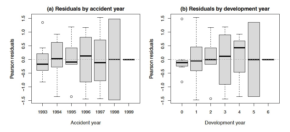
Cell counts range from 2 to 1,914, and the data are genuine integer-valued claim counts. Unlike the Taylor–Ashe paid amounts data, this triangle directly satisfies the micro-level assumptions of Section 4, making the Poisson-mixture micro-level reading of \(\kappa\) fully valid at the cell level. The development pattern exhibits a documented structural drift. Measured on a common basis as the first-development-year share within the first two development years, \(N_{i,0}/(N_{i,0}+N_{i,1})\) rises from \(220/1{,}075 = 20.5\%\) in 1993 to \(485/765 = 63.4\%\) in 1998. (The full-row share for 1993, \(220/2{,}968 = 7.4\%\), is not comparable with the two-cell 1998 figure.) This drift is structured, across-row non-stationarity rather than i.i.d. cell noise. The constant-\(\kappa\) model cannot represent it directly, so \(\hat\kappa\) absorbs it as residual overdispersion. The empirical \(\hat\kappa = 4.8\) therefore conflates genuine cell-level dispersion with this drift, which is exactly why the by-development-year residuals (Figure 2) show a pattern and motivate the time-varying-\(\beta\) extension.

Figure 2.Pearson residuals by factor level for Australian motor bodily injury. (a) By accident year. (b) By development year.

9.1.2. Model fitting

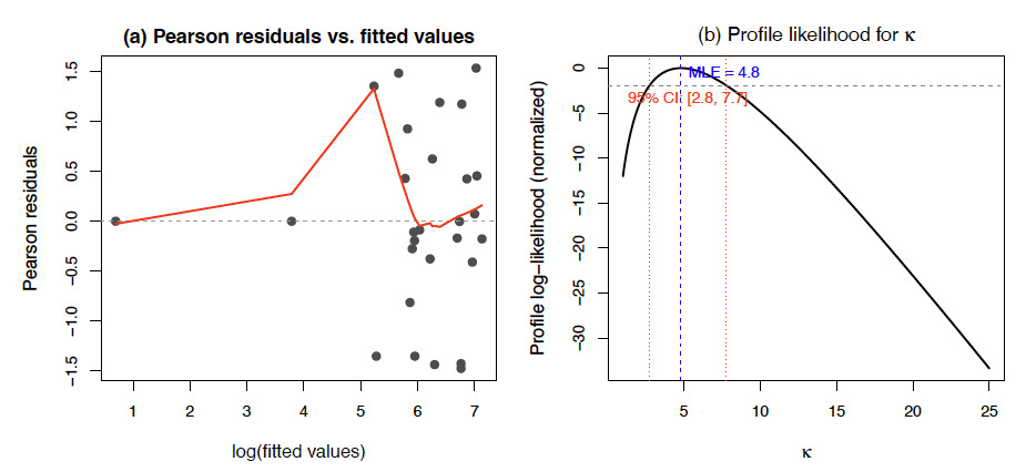
The NB-CL model is fitted using MASS::glm.nb with \(n = 28\) observed cells and \(p = 13\) parameters (intercept, 6 accident-year effects, 6 development-year effects). The estimated dispersion parameter is \(\hat{\kappa}_{\text{MLE}} = 4.8\) with a profile likelihood 95% confidence interval of \([2.8, 7.7]\), indicating substantial overdispersion. The bias-corrected estimate is \(\hat{\kappa}_{\text{adj}} = 4.8 \times (28 - 13)/28 = 2.6\). That \(\hat{\kappa}_{\text{adj}}\) lies below the profile-likelihood interval is not a contradiction: The interval quantifies sampling uncertainty around the uncorrected MLE, whose finite-sample upward bias is precisely what the correction removes.

The likelihood ratio test for overdispersion yields \(\Lambda = 2{,}550.1\) with \(p < 10^{-20}\), overwhelmingly rejecting the Poisson model. The AIC improvement equals \(\Delta\text{AIC} = 2{,}548\), hence the overdispersion parameter is clearly needed.

The dispersion parameter \(\hat{\kappa} = 4.8\) has a direct structural interpretation: The variance of the cell-level shocks is \(1/\hat{\kappa} = 0.21\), a coefficient of variation of \(46\%\) around the fitted multiplicative structure, consistent with the documented instability of the reporting pattern in this portfolio. Under the simplex parameterization of Section 5.2, the estimated accident-year totals \(\hat{\mu}_i = \exp(\hat{\alpha}_i)\) provide a direct readout of the implied ultimate claim count for each accident year, and the development weights \(\hat{w}_j = \exp(\hat{\beta}_j)\) sum to unity by construction.

9.1.3. Reserve estimates

Table 5 presents accident-year reserve estimates with 95% prediction intervals from the NB-CL (corrected) bootstrap with \(B = 5{,}000\) replications.

The coefficient of variation increases for more recent accident years, where a larger proportion of development remains outstanding; it is highest for accident year 1999, which has only one observed cell (two claims in DY 0). The prediction intervals are highly asymmetric: The upper bound for the total reserve (\(7{,}785\)) is 2.4 times the point estimate, while the lower bound (\(1{,}563\)) is 0.5 times, reflecting the right-skewed nature of the negative binomial predictive distribution. This asymmetry would be missed by normal approximations or delta-method intervals.

The total reserve CV of 42.5% is substantial, driven largely by the high cell-level dispersion (\(\hat{\kappa} = 4.8\)) around the fitted development structure and the nonstationary development pattern. For comparison, Mack’s distribution-free model yields a total reserve standard error of 1,612 (CV 50.5%), reflecting Mack’s column-specific variance parameters \(\sigma_j^2\); the NB-CL total CV is thus somewhat lower than Mack’s on this portfolio. Practitioners should note that the development pattern in this dataset is nonstationary (Table 4), which contributes to the large estimated overdispersion.

9.1.4. Diagnostics

Figure 3 shows diagnostic plots for the NB-CL fit. The left panel displays Pearson residuals against log-fitted values. Residuals are centered around zero with no systematic pattern, supporting the log-additive mean structure. The right panel shows the profile likelihood for \(\kappa\). The curve is unimodal and well peaked around the MLE of 4.8, with the 95% confidence interval \([2.8, 7.7]\) confirming that \(\kappa\) is identifiable despite the small triangle size (\(7 \times 7\), 28 cells).

Figure 3.Diagnostic plots for NB-CL fit to Australian motor bodily injury count data. (a) Pearson residuals versus log-fitted values. (b) Profile likelihood for \(\kappa\) with MLE and 95% confidence interval.

Figure 2 displays residuals stratified by accident year and development year. The accident-year panel shows no systematic pattern. The development-year panel reveals a mild drift in residual medians across early development periods, which may reflect the nonstationary reporting patterns documented in the data description—the proportion of same-year finalizations increases substantially from 1993 to 1999. This structure would not be captured by the basic log-additive model and motivates the calendar-year extensions discussed in Section 10.4.

9.2. Benchmark comparison: Taylor–Ashe paid amounts

The Taylor–Ashe triangle (Taylor and Ashe 1983) is the standard benchmark in the reserving literature and is presented here purely for numerical comparison. The NB-CL model is applied as a working approximation; the micro-level derivation of Section 4 does not apply to paid amounts, and a rigorous treatment would require Tweedie GLMs or a frequency-severity decomposition (Wüthrich and Merz 2008).

Fitting MASS::glm.nb to the \(10 \times 10\) triangle yields \(\hat{\kappa} = 13.8\). The classical chain ladder point estimate, equivalently the Poisson CL and ODP CL estimate, is $18.68 million (18,680,856); the NB-CL point estimate is $18.09 million (18,085,795), a \(3.2\%\) departure. This is a concrete instance of the finite-\(\kappa\) point-estimate difference of Section 8.2: The NB2 working weights downweight the high-mean cells relative to the Poisson weights, shifting the fitted development structure. The NB-CL (corrected) interval is \([13{,}288{,}238;\, 24{,}447{,}436]\), compared with the ODP bootstrap interval of \([13{,}400{,}018;\, 25{,}308{,}582]\). The two interval widths are close (11.2M versus 11.9M), consistent with the simulation finding (Table 2) that the gap between NB-CL and the ODP residual bootstrap narrows as overdispersion weakens; at \(\hat\kappa = 13.8\) the two are in the mild-overdispersion regime. The structural conclusions of the paper rest entirely on the Australian motor bodily injury illustration.

10. Discussion

10.1. Interpretability and micro-level consistency

The NB-CL model sets itself apart from quasi-likelihood and moment-based approaches through its interpretability. The micro-level construction of Section 4 derives the negative binomial as the marginal of a Poisson–gamma process in which the gamma shock captures cell-level overdispersion in the incremental counts, i.e., period-to-period fluctuation in the claim-generating environment around the fitted development structure, rather than heterogeneity across accident years, which the free accident-year parameters absorb. As such, the overdispersion routinely observed in claims triangles is not a statistical nuisance to be absorbed by a dispersion parameter, but a quantitative reading of the portfolio’s reporting-pattern instability. This is illustrated by the Australian motor bodily injury example of Section 9.1: The fitted \(\hat\kappa = 4.8\) corresponds to a coefficient of variation of \(1/\sqrt{\hat\kappa} \approx 46\%\) in the cell-level shocks around the fitted development pattern. That figure is inflated by the structured reporting-pattern drift documented in Section 9.1, which the constant-\(\kappa\) model absorbs rather than represents; what \(\kappa\) does not measure is heterogeneity across accident-year intensities, which the free accident-year effects absorb.

The ODP and Mack models reproduce the chain ladder point estimates, and in moderate-\(\kappa\) regimes, variance estimates of broadly similar magnitude to the NB-CL ones (though on the Australian portfolio Mack’s total CV is the larger; Section 9.1). Neither model explains, however, why the assumed variance structure should hold. Note that this is not a numerical limitation but a structural one: A variance assumption without a generative model is difficult to validate and to extend.

10.2. Uncertainty quantification

The NB-CL model provides coherent predictive distributions via the parametric bootstrap. Unlike the residual (ODP) bootstrap, which resamples Pearson residuals, the NB-CL bootstrap resamples from a fully specified distribution. This ensures consistency between the assumed model and the uncertainty quantification procedure.

The variance decomposition equation (7) explicitly separates process and estimation variance, mirroring the structure of Mack (1993) and Merz and Wüthrich (2007) but arising from a likelihood-based framework. The accident-year-level prediction intervals in Table 5 illustrate the practical value of this decomposition, showing how uncertainty varies across accident years as a function of the remaining development.

10.3. Limitations

The NB-CL model has four limitations.

The micro-level derivation in Section 4, i.e., Poisson arrivals with gamma heterogeneity yielding negative binomial counts, is rigorous for incremental claim counts. When applied to incremental paid amounts, as is common in actuarial practice, the NB-CL model should be viewed as a convenient working approximation rather than a structural likelihood. For a principled treatment of claim amounts, Tweedie GLMs (Wüthrich and Merz 2008) or frequency-severity decompositions provide more appropriate foundations.

The classical chain ladder development factors can be computed in closed form from cumulative column totals, without iterative optimization. The NB-CL model, formulated as a GLM, requires iterative estimation via iteratively reweighted least squares. While modern software makes this computationally trivial, practitioners who value closed-form expressions may find this less appealing. In the Poisson limit \(\kappa \to \infty\), however, the NB-CL maximum likelihood estimators coincide with the classical marginal-totals estimators, so the connection is not entirely lost.

The log-additive structure assumes that development-year effects are constant across accident years, which may not hold in portfolios undergoing structural changes, as illustrated by the nonstationary development pattern in the Australian motor bodily injury data (Section 9.1). The model also assumes independence across cells, which may be violated in the presence of calendar-year effects or operational changes. The misspecification study (Section 8.3) shows that unmodeled calendar-year effects produce the most concerning degradation in coverage (92% versus nominal 95%), while development-varying dispersion is relatively benign (95%). Finally, the model assumes a single dispersion parameter \(\kappa\) for all cells, whereas in practice, dispersion may vary by development year or calendar year.

10.4. Extensions

Four natural extensions remain. Allowing \(\beta_j\) to vary across accident years would capture structural changes in reporting behavior. Adding a calendar-year term \(\gamma_{i+j}\) to the linear predictor would accommodate superimposed inflation. A Bayesian NB-CL model with priors on \((\pmb{\alpha}, \pmb{\beta}, \kappa)\) would provide posterior inference and natural regularization for sparse triangles and is the theoretically preferred uncertainty quantification procedure: It propagates parameter uncertainty through the posterior rather than approximating it via a profile likelihood correction, thereby eliminating the need for the bootstrap entirely. Empirical validation is still needed, particularly for small triangles where estimation uncertainty in \((\pmb{\alpha}, \pmb{\beta})\) is large relative to triangle size. Joint modeling of multiple lines of business via copulas or hierarchical random effects, and integration with micro- or macro-level severity models, would together extend the NB-CL frequency model into a fully stochastic multiline reserving framework.

The Bayesian NB-CL model is closely related to the exact Bayesian model of Wüthrich and Merz (2008), Section 4.3.1, in which the authors place a gamma prior on the Poisson mean in the ODP framework and derive the negative binomial as the exact marginal distribution. The NB-CL model can therefore be viewed as the frequentist profile likelihood counterpart of their Bayesian conjugate analysis: Both yield the same marginal distribution for incremental counts, but the NB-CL dispersion parameter \(\kappa\) is estimated by maximizing the adjusted profile likelihood rather than treated as a hyperparameter of the gamma prior. Under a flat prior on \(\kappa\), the two approaches coincide asymptotically; for small triangles, the Bayesian formulation with an informative prior on \(\kappa\) is the theoretically preferred procedure, as it propagates hyperparameter uncertainty through the posterior rather than conditioning on a point estimate.

11. Conclusion

The classical chain ladder method has no likelihood, and its two main stochastic companions each fall short on a different front: The Mack model stops at the second moment, while the ODP framework rests on a quasi-likelihood variance structure without a generative interpretation. The NB-CL model fills the latter gap. Incremental counts are modeled as negative binomial with a log-additive mean, the resulting MLEs coincide with the chain ladder estimators in the Poisson limit, and the dispersion parameter \(\kappa\) is given a structural reading via the micro-level Poisson–gamma construction of Section 4. \(\kappa\) is the inverse variance of the cell-level gamma shocks around the fitted mean structure, thereby turning what is usually treated as a statistical nuisance into an interpretable portfolio characteristic.

As shown in Section 7, within the chain ladder family, only the Poisson CL model is an exact special case of the NB-CL likelihood: The ODP model approximates it only locally, while the Mack model merely shares its point estimates. This positioning clarifies the assumptions underlying the classical reserving methods.

Estimation of the NB-CL model can be performed using standard GLM techniques, with the dispersion parameter estimated via the adjusted profile likelihood. A parametric bootstrap procedure incorporates both process and estimation variance, yielding well-calibrated predictive intervals. Simulation studies demonstrated that the NB-CL model achieves nominal coverage under correct specification and degrades gracefully under model misspecification, with the exception of unmodeled calendar-year effects, which produce modest undercoverage and should be checked in practice.

Empirical illustrations on both claim count data (Australian motor bodily injury) and paid amounts data (Taylor–Ashe) confirmed that the model fits both data types without numerical difficulty. The claim count illustration, where the micro-level assumptions hold exactly, demonstrated the structural interpretation of \(\kappa\) as cell-level shock dispersion, with the portfolio’s documented reporting-pattern instability as its visible source. Heterogeneity at the accident-year level, by contrast, is absorbed by the free accident-year parameters and requires anchored or hierarchical levels for identification (Remark 2).

Time-varying development patterns, calendar-year effects, the Bayesian formulation, and frequency–severity coupling still need to be investigated. Section 10.4 sketches the corresponding entry points.

Acknowledgments

The author thanks Michel Denuit for helpful comments on an earlier version of this paper.

Use of generative AI

A large language model (Anthropic’s Claude) was used as an assistive tool during the preparation of this manuscript. All scientific content is the author’s own, and the author takes sole responsibility for it.