
The paper presents a recursive extension of the Bornhuetter–Ferguson (BF) approach for estimating ultimate loss ratios. The method proposed follows the Bayesian tradition: New information updates prior expectations, but only to the extent that the observed result is plausible given the model’s existing view of the world.
A key goal of all loss-reserving methods is to balance stability based on prior expectations with responsiveness to emerging experience. Some methods tend to emphasize responsiveness, while others tend to emphasize stability. The chain ladder (CL) method is very sensitive to loss development patterns and may therefore overreact to volatility or sparse data. The BF method anchors to an expected loss ratio (ELR) and may provide stability at the cost of slower adaptation to real differences in underlying assumptions. Recursive approaches (Benktander 1976) have been proposed to address this tension by updating the BF prior over time. Other authors have suggested a credibility-weighting of methods (Robbin 1987; Mack 2000; England and Verrall 2002; Verrall 2000).
The proposed framework extends the BF method by replacing a fixed ELR with a dynamically updated estimate at each development period. The update is determined by using the BF-implied ultimate loss ratio (ULR) as a probe, at each valuation, within a parametric loss ratio distribution. The signal sent back by the probe is used to evaluate the plausibility of the BF-implied ULR under the assumed loss ratio distribution. A systematic adjustment is then made to the a priori ELR, and the volatility of the loss distribution is attenuated as the accident year ages.
Simulation results demonstrate that the method performs well across a range of volatility and development regimes. While it does not uniformly dominate traditional CL or BF approaches, it frequently produces more accurate ULR estimates in environments characterized by unstable reporting patterns or elevated loss ratio volatility. It converges naturally toward traditional estimates as development matures. The framework is designed for practical implementation using standard actuarial tools (i.e., Excel, Python) and is intended to complement, rather than replace, existing reserving methods.
1. Introduction and motivation
Estimating ULRs is a central task in property and casualty reserving, requiring actuaries to balance stability derived from prior expectations with responsiveness to emerging experience. Traditional reserving methods approach this balance in different ways. The chain ladder (CL) method (alternatively referred to as the loss development factor, or LDF, method) relies on loss development factors derived from reported loss emergence patterns, allowing estimates to adjust quickly but potentially overreacting to volatility or anomalous experience. The Bornhuetter–Ferguson (BF) method, by contrast, emphasizes an ELR, providing stability at the cost of slower adaptation when actual experience differs from expectations.
In practice, actuaries face uncertainty in both the selected ELR and the selected loss development pattern. Either assumption may prove inaccurate because of parameter misestimation, process variation, or some combination of the two.
Bayesian approaches offer a natural conceptual framework for balancing prior beliefs and observed data. However, fully specified Bayesian reserving models often require detailed likelihood assumptions and computational techniques (e.g., Wüthrich and Merz 2008).
This paper proposes a pragmatic extension of the BF method that incorporates distribution-based updating in a form that remains transparent and implementable using standard actuarial tools. By modeling ULRs through a parametric distribution and introducing a probability-based weighting mechanism that moderates the influence of emerging experience, the proposed framework seeks to provide another viewpoint in addition to traditional approaches.
2. Background and literature context
The BF method occupies a central position in actuarial reserving practice, particularly for lines of business with significant reporting lags. By combining reported losses with an expected ultimate loss estimate weighted by the proportion of losses yet to be reported, BF provides a structured approach to reserving under uncertainty (Bornhuetter and Ferguson 1972).
Extensions of BF include approaches that update the BF prior over time, such as the iterative method of Benktander (1976), as well as approaches that blend BF with other reserving estimates.
Bayesian reserving methods have been explored in the actuarial literature, often focusing on modeling claim counts, severities, or aggregate losses within a probabilistic framework (England and Verrall 2002; Wüthrich and Merz 2008). These approaches provide a coherent treatment of uncertainty and a principled mechanism for combining prior information with observed data.
Credibility theory provides another lens through which to view the balance between prior expectations and emerging experience (Bühlmann 1967; Hachemeister 1975). Classical credibility approaches formalize the weighting of different information sources based on their relative reliability. However, translating classical credibility formulations directly to loss development settings is not straightforward. Credibility models require clearly defined units of observation, repeated independent data, and estimable variance components, none of which map naturally to development triangles, where observations across development periods are dependent and the appropriate definition of exposure and sample size is ambiguous. As a result, credibility is typically applied in practice to blend different reserving estimates or external benchmarks, rather than directly within the loss development process itself. For example, Robbin (1987) describes credibility-weighted combinations of BF, CL, and initial loss ratio estimates.
The framework proposed herein draws on elements from these traditions. It preserves the intuitive structure of the BF method and incorporates probabilistic ideas through an explicit loss ratio distribution that is evaluated and implicitly revised at each development period. Unlike approaches that combine BF with other reserving estimates through credibility weighting, the proposed method derives a BF estimate using a recursively updated a priori ELR. In this formulation, the weighting factor is not an externally specified credibility parameter; it is derived from the probability assigned to the BF-implied ultimate under the assumed loss ratio distribution. In doing so, the method seeks to bridge the gap between theoretical rigor and practical applicability.
3. Methodology: A distribution-based recursive extension of the BF method
3.1. Loss ratio distribution framework
This section describes the construction of the prior belief distribution for the ULR used in the examples that follow. The lognormal assumption is illustrative; any suitable distribution may be used.
The proposed method models the ULR as a random variable following a parametric distribution, assumed here to be lognormal. In practice, one common actuarial approach to parameterizing a loss ratio distribution begins with the development of a claim severity cumulative distribution function, often constructed by blending exposure-based and experience-based severity information. An ELR is then determined through standard actuarial adjustments to historical experience, including trend, on-leveling, and other pricing considerations. Given an expected premium amount, the ELR, and the average claim severity implied by the severity distribution, an expected claim frequency is derived and modeled using a discrete frequency distribution, typically Poisson or negative binomial. Aggregate loss ratios are generated through simulation by combining the severity distribution with the frequency model, producing an empirical distribution of ULRs, which can then be fit to a parametric form such as the lognormal distribution. Alternative modeling approaches and distributional choices are possible, but consideration of those extensions is beyond the scope of this paper.
3.2. BF benchmark
At each development period, a BF-implied ULR is calculated using the prior ELR and the loss development factor for that valuation. This BF-implied ULR estimate serves as a probe into the assumed parameterized loss ratio distribution.
3.3. The BF-implied loss ratio as a plausibility probe
To formalize the updating mechanism, define:
Et=expected (a priori) ultimate loss ratioRt=actual reported loss ratioLDFt=selected loss development factorBt=BF-implied ultimate loss ratioCt=conditional expectation between Et and BtPt=tail probability (plausibility measure)Ht=plausibility-adjusted a priori estimateULR=ultimate loss ratio
That is,
The relative plausibility of under the prior loss ratio distribution is used to assess the consistency of the emerging experience with prior expectations. This plausibility measure governs the influence of new information on the updated ULR estimate
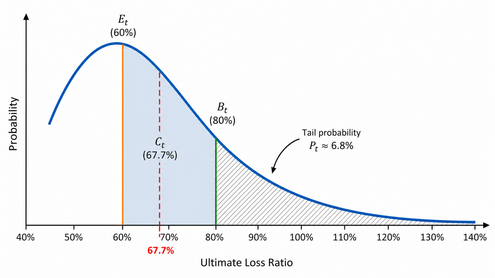
In this paper, denotes a probability mass under the ULR belief distribution, defined as the tail probability of observing an outcome at least as extreme as may be expressed as the smaller of the two tail probabilities around Mathematically, so that by construction. We interpret this probability as governing the weight applied to the prior expected ULR with the complementary weight applied to the conditional expectation Accordingly, while the mechanics of the method operate entirely in probability space, the resulting probability determines the weighting applied in the update.
This probability reflects the degree to which the emerging experience is consistent with the prior belief distribution. When lies in a region of high probability under the prior distribution, the observed experience is broadly aligned with prior expectations, and the update remains close to the prior estimate. Conversely, when lies in the tail of the distribution, the observed experience is less consistent with prior beliefs, and the update moves further away from the prior toward the conditional expectation. In this way, the weighting is determined directly by the degree of agreement between emerging experience and the prior distribution, rather than specified exogenously. As this agreement increases, moves closer to the prior, and the resulting movement from the current diminishes. In the limiting case where coincides with the a priori estimate, the associated tail probability approaches 50%. In this case, converges to the prior, and the updated estimate remains unchanged, as would be expected intuitively.
The conditional expectation over the region between the a priori ULR and determines both the direction and magnitude of the update (labeled conditional in Figure 1). By intention, low plausibility produces a stronger adjustment away from the prior, while higher plausibility produces a more modest adjustment.
Unlike the classical BF method, which reuses a fixed ELR at each development period, the proposed framework updates the a priori ELR recursively. In this way, adverse or favorable signals influence future estimates gradually through accumulation over time rather than through abrupt adoption or complete disregard.
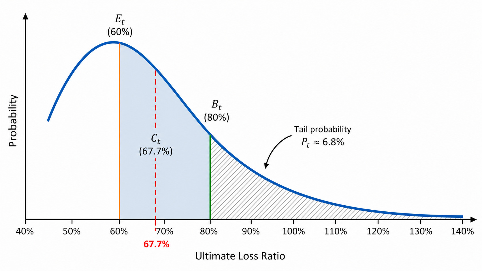
Figure 1 is intended as a conceptual illustration of the updating mechanics for a single development period. In practice, this procedure is applied iteratively across development periods, with the parametric loss ratio distribution’s volatility decaying as reporting matures, as described in the sections that follow.
This relationship can be expressed explicitly through the updating formula. Formally, define
Ht=Pt×Et+(1−Pt)×Ct.
Although Equation 1 resembles a credibility formula, is not a classical credibility weight. In classical credibility applications, the credibility assigned to observed experience generally increases with the volume or reliability of the experience. Here, is a tail probability measuring the plausibility of the BF-implied ULR under the current belief distribution.
Then as defined in Equation 1, serves as the a priori estimate in computing The update may be expressed as a probability-weighted adjustment applied to the unreported portion of the estimate, preserving the BF structure while modifying the expectation underlying that portion.
Let denote the expected ULR under the belief distribution at development period and let denote the conditional expectation illustrated in Figure 1. The updated expected ULR at development period is then given by Equation 2.
Et+1=Rt+(1−1/LDFt)×Ht.
Worked example. Suppose that at development period the prior expected ULR is the actual reported loss ratio is and the selected loss development factor is The corresponding BF-implied ULR is as follows:
Bt=Rt+(1−1/LDFt)×EtBt=50%+(1−1/2.0)×60%Bt=50%+0.5×60%Bt=80%.
Under the current belief distribution, the conditional expectation between the prior expected ULR and is and the tail probability assigned to is The plausibility-adjusted a priori estimate is therefore
Ht=Pt×Et+(1−Pt)×CtHt=0.068×60%+0.932×67.7%Ht=4.1%+63.1%Ht=67.2%.
The updated expected ULR is then
E(t+1)=Rt+(1−1/LDFt)×HtE(t+1)=50%+(1−1/2.0)×67.2%E(t+1)=50%+0.5×67.2%E(t+1)=83.6%.
The plausibility-weighted estimate is not substituted for the ULR, but instead is used within the traditional BF structure. Consequently, the updated estimate may exceed both and
The calculation of the conditional expectation and tail probability from the underlying loss ratio distribution is illustrated in Appendix A.
3.4. Recursive updating and volatility attenuation
The proposed method is implemented as a recursive algorithm, applied at each development period. The resulting becomes the for the subsequent development period in the BF plausibility probe.
The parameterized loss ratio distribution is also updated. The mean is re-centered around the new ULR estimate The assumed standard deviation of the distribution decreases as development progresses. The degree of attenuation is explicitly linked to the loss development factor and bounded by a selected minimum retained proportion to prevent unrealistic overconfidence.
Let denote the initial standard deviation parameter and let denote the minimum proportion of retained at later development periods. The updated standard deviation parameter is defined in Equation 3.
σt+1=σ0×[w+(1−w)max(1−1LDFt,0)].
Here, is a selected weighting parameter rather than a separately derived estimate of volatility. It determines the minimum proportion of the initial standard deviation retained as development matures, while the remaining portion of the standard deviation attenuates with the unreported proportion implied by the selected loss development factor. Thus, the formula should be understood as a modeling assumption for reducing distributional uncertainty over time, not as a uniquely derived actuarial result. Other reasonable attenuation functions could be selected based on the actuary’s judgment, the volume and volatility of the data, and the intended application.
Although volatility is higher early in development, this is expected when the data is still immature. At this stage, differences between and are more likely to reflect noise than meaningful signal. Under the method presented in this paper, this is handled mechanically: Higher volatility produces a wider distribution with heavier tails, which makes large deviations more plausible and therefore assigns greater weight to
As development progresses and volatility declines, the distribution narrows, deviations become less likely to occur by chance, and the method responds more strongly to divergent observations. Appendix B extends this example across multiple evaluation periods, showing how the same distance between and may receive different treatment as the accident year matures and the assumed volatility declines.[1]
This formulation preserves the familiar structure of the BF method while introducing an explicit, distribution-based plausibility mechanism that recognizes, yet moderates, the influence of emerging experience.
4. Simulation design
The proposed method is evaluated using a simulation framework designed to compare its performance with traditional CL and BF approaches across a range of volatility and development regimes.
A regime refers to the fixed inputs used for a simulation. In each iteration, randomness is introduced through both the simulated ULR and the loss development pattern, while all other inputs—such as the ELR, the expected loss development factors, and the loss ratio distribution—remain the same. Regimes differ primarily by the level of prescribed volatility. Reported loss ratios are derived from the simulated ULR and the simulated loss development pattern for each iteration.
Several regimes are considered, including scenarios in which development patterns align closely with assumptions at one extreme, and scenarios characterized by substantial volatility at the other. Performance is evaluated across multiple dimensions—including accuracy, bias, stability, catastrophic misses, and tail behavior—using a rank-based composite score (discussed in Section 5), with root mean squared error (RMSE) reported separately to assess single-metric dominance.
Simulation of emergence volatility
Reported loss emergence is simulated by perturbing an expected emergence path with increasing levels of random variation. In the baseline case (volatility level 0), reported losses follow the deterministic expected emergence implied by the loss development factors.
For positive volatility levels, expected emergence at each development period is multiplied by a random factor drawn from a normal distribution with mean one and standard deviation equal to the volatility level expressed as a percentage. For example, a volatility level of 10 corresponds to a one-standard-deviation variation of approximately around expected emergence.[2]
Reported losses are constrained to be nondecreasing across development periods and are capped at the simulated ultimate loss for each path. Volatility levels ranging from 5 to 100 are evaluated, representing increasingly noisy reporting behavior around an otherwise fixed development pattern.
For example, if the expected reported loss in a given period is 100, a volatility level of 10 would typically produce outcomes in the range of about 90 to 110, reflecting modest variation around the expected path. In contrast, a volatility level of 100 would allow for much larger swings, with outcomes that could vary widely around 100, such as 50 or 150, reflecting highly unstable reporting behavior.
5. Results
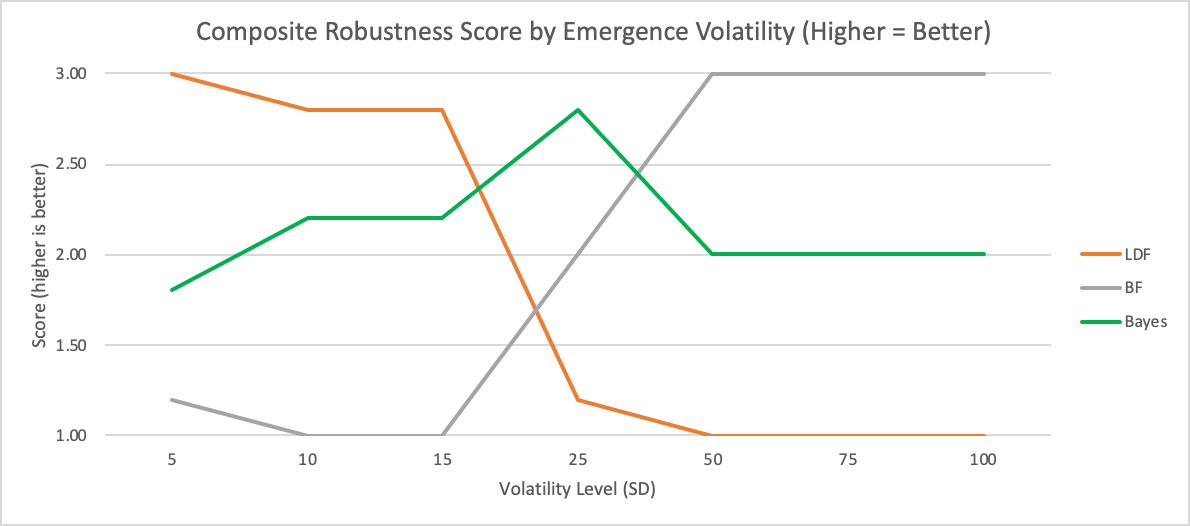
To evaluate performance across reserving methods, this paper introduces the composite robustness score, or CR score. The CR score is a composite, rank-based metric that aggregates relative performance across bias, error, and volatility diagnostics, as described in Appendix C. For each volatility level, methods are ranked across those dimensions, and the resulting ranks are combined into a single score.
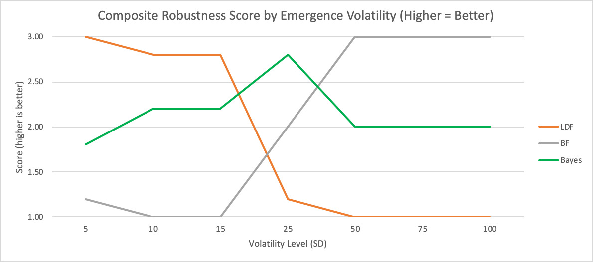
As Figure 2 shows, relative performance varies systematically with volatility. Under conditions of low volatility (loss emergence closely aligned with CL (LDF)–implied expectations), the CL method produces the most favorable CR score. Under conditions of high volatility (substantial divergence from implied loss emergence patterns), the BF method produces the most favorable CR score, consistent with its comparatively conservative reliance on a stable ELR. The proposed method, referred to as the Bayesian plausibility method here, remains consistently competitive across regimes, with its strongest relative standing occurring at moderate volatility and second-place rankings at the volatility extremes. These results indicate that no single method dominates universally; rather, the CR score ordering depends on the degree of volatility.
To complement the rank-based CR score comparison in Figure 2, Table 1 reports RMSE by method across the same regimes. RMSE is the square root of mean squared error and is expressed in loss ratio percentage points, making it easier to interpret than MSE, which is measured in squared loss ratio units.
Table 1 reports RMSE by method across the same volatility regimes. The results show a clear progression across regimes. At low volatility levels, the CL method produces the lowest RMSE because reported emergence remains close to the selected development pattern. As volatility increases, the Bayesian plausibility method begins to outperform both traditional methods, reflecting its ability to respond to emerging experience without fully adopting the volatility of the CL estimate. At higher volatility levels, BF remains competitive because its fixed ELR anchor protects it from noisy emergence. At the highest volatility level, however, the Bayesian plausibility method again produces the lowest RMSE, suggesting that BF’s fixed anchor can become too rigid when the implied ULR provides a sufficiently strong signal that the original selected ELR may no longer be appropriate. This pattern illustrates the intended role of the proposed method: It does not replace CL or BF in all regimes but occupies the middle ground between responsiveness and stability, adapting as the reliability of emerging experience changes.
6. Discussion
Building on the empirical results presented in Section 5, this section interprets the observed regime-dependent behavior and discusses the implications of probability-weighted updating relative to classical methods.
6.1. Interpretation of regime-dependent performance
The proposed Bayesian plausibility method performs most effectively in environments where emergence deviates meaningfully from the implied development pattern but is not dominated by noise. In such moderate-volatility regimes, the method incorporates emerging information when it is plausibly informative while continuing to moderate updates through the prior distribution.
At the extremes, performance aligns with intuition. When emergence closely follows the implied development pattern, methods that rely directly on those patterns perform best. Conversely, when emergence is highly volatile, methods that anchor more heavily to prior expectations provide greater stability. The proposed framework adapts between these regimes, producing consistently competitive results across a broad range of conditions.
6.2. Robustness versus optimality
A key insight from the simulations is that robustness, rather than pointwise optimality, is the primary advantage of the proposed method. While CL and BF each excel in specific regimes, their performance deteriorates when applied outside those regimes. In contrast, the proposed method is generally competitive across the volatility levels tested, rarely producing the worst outcome and performing particularly well in several regimes where emergence behavior is uncertain.
From a practical reserving perspective, this distinction is important. Actuaries rarely know ex ante which emergence regime will prevail. Methods that perform well only under narrowly defined assumptions may introduce unintended volatility or bias when those assumptions fail. A method that performs consistently well across a broad range of scenarios may therefore be preferable, even if it is not optimal in every case.
6.3. Relationship to credibility principles
The weighting mechanism underlying the proposed framework is related to classical actuarial credibility principles, but it is not a classical credibility formula. Rather than introducing an explicit credibility parameter the method determines the relative weight assigned to prior expectations and emerging experience through a plausibility measure derived from the loss ratio distribution. In this sense, new information is incorporated in proportion to its reliability, with the weight emerging endogenously from the model rather than being specified exogenously.
6.4. Practical implications for reserving practice
The proposed framework is best viewed as a complement to existing reserving methods rather than a replacement. It may be particularly useful for long-tailed lines of business, early accident year evaluations, or portfolios exhibiting unstable or evolving reporting patterns. In such settings, the method provides a structured and transparent way to balance prior expectations with emerging experience without relying exclusively on either.
Because the framework can be implemented using standard actuarial tools and does not require fully specified likelihood models or advanced Bayesian computation, it is accessible to practitioners and suitable for routine reserving workflows. Appendix D provides a step-by-step implementation guide for readers who wish to apply the method in practice.
In practice, classical methods are often applied in a maturity-dependent manner: The CL method is called upon for more mature accident years as loss development factors approach unity, while BF is frequently relied upon for less mature years where emergence is more volatile. The proposed framework operates along a different axis. Its primary strength is not tied to accident year maturity per se, but to situations in which the practitioner is concerned about potential systematic biases in either the ELR or the selected development factors.
6.5. Limitations and future extensions
A central feature of the proposed framework is its intentional agnosticism with respect to both the choice of ULR distribution and the choice of development-period ultimate estimator used to assess plausibility. The lognormal distribution and the BF estimate are employed in this paper for their familiarity and interpretability, not because the plausibility mechanism depends on either choice. Any actuarially reasonable parametric or semiparametric ULR distribution may be used, and any method that maps reported experience to a development-period implied ultimate—such as loss development–based, Cape Cod, or hybrid estimators—may serve as the plausibility probe. The contribution of this paper lies in the plausibility-based structure itself, which operates independently of these modeling choices and remains invariant under their substitution.
The weights employed in this framework are intentionally defined in probability space, based on the plausibility of a development-period implied ultimate under the current ULR distribution. This formulation is heuristic in the actuarial sense: It is designed for transparency, interpretability, and practical implementation rather than derived from an explicit likelihood for reported losses. The objective is not to construct a fully specified Bayesian reserving model, but to introduce a distributionally informed probability mechanism that can be implemented using standard actuarial tools and professional judgment.
The simulation framework is also stylized by design. It focuses on uncertainty in development-period loss emergence and does not explicitly model calendar year influences, changes in claims handling or reserving practices, or shifts in reporting behavior that render historical loss development factors unrepresentative of future experience. Such effects are well recognized in practice and are typically addressed through separate diagnostic and judgmental processes; incorporating them directly would represent a distinct modeling objective beyond the scope of this paper.
Future research could extend the framework in several orthogonal directions, including the use of alternative ULR distributions, exploration of different mappings from plausibility to probability, or integration with models that explicitly address exposure changes, claim frequency dynamics, or evolving reporting patterns. Such extensions would build upon the plausibility-based structure presented here but are intentionally left outside the present scope in order to maintain focus on the reserving mechanics of dynamic probability weighting.
7. Conclusion
The paper introduces a probability-weighted Bayesian extension of the BF method that incorporates an explicit loss ratio distribution and a dynamic plausibility mechanism for updating ULR estimates over time. The approach is motivated by a practical reserving challenge: balancing the stability of a priori expectations with appropriate responsiveness to emerging experience in the presence of reporting volatility.
The principal contribution of the framework lies in its robustness. By evaluating emerging experience through the lens of a prior distribution and moderating updates through an explicit plausibility mechanism, the method adapts to changing emergence conditions without overreacting to noise or anchoring excessively to prior assumptions. This behavior is informed by actuarial credibility principles and provides a transparent, interpretable structure for dynamic updating.
Importantly, the method is designed for practical implementation. The framework can be implemented using spreadsheet-based or lightweight scripting tools (e.g., Excel or Python). As such, it is intended to complement existing reserving approaches and to provide practitioners with an additional perspective when uncertainty regarding emergence behavior is material.
Acknowledgments
The author thanks Steve White and Cameron Vogt for informal discussions and practitioner feedback that helped refine certain modeling choices. The author thanks members of the CAS Loss Reserving Project Oversight Group for their review and helpful comments. All remaining errors, interpretations, and conclusions are solely the responsibility of the author.