Data Quality and Validation for Reserving Data Pipelines

undefined

1. Introduction

Ensuring high data quality has long been recognized as an essential part of all actuarial work, having a direct impact on an insurer’s ability to meet its obligations, comply with regulatory standards, and enable long-term profitability. The topic of data quality can be quite broad, so this paper narrows its scope to focus on what high-quality data means in the context of an actuarial reserve analysis and how an actuary identifies whether their dataset is suitable for the intended purpose. The paper discusses how to determine the desirable properties of an analytical dataset, how to validate the dataset to confirm that these properties exist (and that undesirable properties are absent), and how best to automate these validation checks within a data pipeline. However, data cleaning is not discussed in great detail. Many common approaches to cleaning, such as imputation and treatment of outliers, are often subjective and may require carefully documented actuarial judgment, given regulatory expectations. These decisions are outside the scope of this paper.

The goal of this text is to share solutions and best practices that address the recurrent pain points and common pitfalls associated with data quality. The end result of adopting these best practices should be fewer surprise data errors, faster and more comprehensive identification of problems, and smoother collaboration with upstream data maintenance teams. Several examples using synthetic datasets are provided to demonstrate how to identify and address various issues early in the reserving process. The datasets and scripts are shared on GitHub with the hope that practitioners may take inspiration from the provided Python and SQL code samples for their own work. Recognizing that teams may use different software stacks, the examples shown are designed to be easily adaptable for other platforms or pipelines. References to third-party tools and open-source packages are intended only for illustrative purposes and do not constitute an endorsement or recommendation by the author.

2. Data quality dimensions

A number of common themes recur across past research studies on data quality standards. There are many ways to categorize problems with a dataset, but the most common taxonomy defines six dimensions:

• Accuracy: Are the values in the dataset correct? Do they reconcile against other sources of truth? For a reserving dataset, the values may reconcile against the general ledger or a claims administration system.

• Completeness: Does the dataset include all relevant information? Do some records have missing values in essential fields? Are all relevant records included in the dataset? In particular, an actuary might want to verify that the data pull includes loss data for all accident years used in an analysis.

• Consistency: Are the records in the dataset consistent with each other? Do values in the dataset match other data sources that contain the same information? For example, if claim ID appears multiple times in a dataset (perhaps once per claimant), it may be reasonable to expect the accident date in each matching record to be the same. Consistency is also essential in defining join criteria when merging two tables.

• Uniqueness: Does the dataset contain duplicated data in some form? This could include, for example, claim numbers appearing twice in the dataset, or a prior step in a data pipeline double-counting the loss amounts for a set of claim numbers before aggregation.

• Validity: Do the fields in the dataset have the appropriate data types? Do the values span an appropriate range? An analyst can set the expectation that loss amounts are rounded to the penny or that the line-of-business field can take only one of five prespecified values.

• Timeliness: Is the data accurate as of a specified point in time? Were there delays in acquiring the data? A quarterly reserve analysis might pull the latest data as of the end of a quarter (March 31, June 30, September 30, December 31). This valuation date should be strictly respected, and the analysis must not include transactions occurring after that point.

There are some interdependencies in these dimensions. For example, resolving an accuracy issue may improve completeness and consistency. There can also be some subjectivity in how a dataset is assessed under these dimensions. As the remainder of the paper builds out a list of validation checks, each one will be mapped to at least one of the dimensions listed above.

3. Data file formats

The format in which data—whether raw or transformed—is stored can be a major source of data issues. Instead of recommending any one universal data format, this section will demonstrate why it is important to be intentional about data formats. Table 1 describes some common file formats that are used in reserving, along with potential advantages and disadvantages.

The most common data quality risks relating to file formats occur due to context loss and file format changes. A file format loses context when it does not preserve relevant metadata (i.e., context) and requires a downstream user to infer information such as data type, origin, and definition of fields. Of the options presented in Table 1, only parquet files and database-specific storage formats are likely to preserve data types natively. For the other formats, such as a comma-separated values (CSV) file, context loss can pose a risk when loading in the file as part of a data pipeline. Many software programs offer convenient functionality that automatically infers an appropriate data type for each column, rather than requiring the user to specify the type for each column. To illustrate the problem with this feature, we can load the same dataset in CSV form and parquet form into Python’s pandas package and examine the difference. The insurance_claims dataset has a column named ‘ncap_rating’ that designates a numeric rating from the National Highway Traffic Safety Administration’s New Car Assessment Program (NCAP). Most vehicles will have an NCAP score associated with them, but very rarely some types of vehicles will receive an “NR” when the model has not been rated.

df = pd.read_csv('Datasets/insurance_claims_ncap.csv')
display(df['ncap_rating'].unique())
Output: array([3, 4, 0, 5, 2, '3', '2', '5', '0', '4', 'NR'], dtype=object)

In the snippet above, the pandas package reads in the first set of rows, automatically recognizes all the column’s values in that sample as integers (0 through 5) and assumes that the rest of the values in that column are also all of integer type. However, when it loads in a later chunk of rows and encounters the string “NR” for the first time, pandas revises all future values in that column as strings, which leads to the column having mixed typing. Trying to filter on a particular ‘ncap_rating’ in a later step runs the risk of unintentionally excluding some integer or string values. A parquet file does preserve data type information when saved, so pandas will correctly determine that the whole column should be represented as a string.

df = pd.read_parquet('Datasets/insurance_claims_ncap.parquet')
display(df['ncap_rating'].unique())
Output: ['3', '4', '0', '5', '2', 'NR']

Along a similar vein, any step in a data pipeline that converts between file formats can lead to misinterpretation of data types. Excel is notorious for automatic conversions of values—opening a CSV file containing zip codes in Excel will strip out leading zeros from valid zip codes, turning 06103, for example, into 6103. Date values originally formatted as “M/D/YY” will be saved as “M/D/YYYY” when edited in Excel, which could break hard-coded date parsing logic in other software.

None of the file format options listed in Table 1 would support other pertinent metadata such as field definitions or data provenance, so data teams usually maintain a data dictionary with this information. When working with CSV files, users should strongly consider leveraging this data dictionary to explicitly specify appropriate data types to avoid the risk of a program making the wrong type inference. In some cases, the discrepancies can be subtle enough that they will not be noticed until a much later step, if at all. An example using pandas’ read_csv function is shown in csv_parquet_import_comparison.ipynb.

Ensuring that an import uses the appropriate data types supports the validity dimension of data quality.

4. Desirable qualities of a data pipeline

This section will cover the following five best practices for designing a robust data pipeline for a reserve analysis:

• Guarantee reproducibility

• Embed validation checks

• Log metrics over time

• Maximize automation

• Plan for extensibility

4.1. Guarantee reproducibility

There will be times when practitioners must revisit a prior reserve analysis and reconstruct the dataset used. This could be to correct an issue with the analysis, backtest a new technique, or comply with an audit. While one approach would be to simply archive the final dataset, it may be difficult to fully explain how some calculations were derived if the pipeline was not preserved.

One effective way to ensure reproducibility across a workflow is to use version control software whenever possible. Git is the most popular solution that allows teams to save any form of text or code files (including .py, .r, .sql, and .sas) in a shared repository. Some of Git’s features include the ability to preserve all code changes with time stamps and the ability to accompany code changes with commit messages (serving as documentation). This allows teams to identify the code that was in use as of a particular run. Any corrections made to the code since it was last used are also easily identifiable.

Enterprise software platforms built on Git include GitHub, GitLab, and Bitbucket, and these platforms offer even more functionality, such as the ability to use pull requests for code reviews and integration with automated testing frameworks. Using Git for large datasets or model artifacts (such as .sas7bdat or .pkl) is usually inadvisable because it may slow down Git’s functionality. These files are best stored in a dedicated data management system.

In addition to requiring that the original code be available, reproducibility also requires that all input data be static and preserved. There may be some types of reserving analyses that invoke another external service or model, and this data must be preserved as well. For example, if a process requires running a claims-level dataset through a neural network model, the neural network model should also be archived. If the model is maintained by an external third party and not directly available, it may be necessary to preserve a time-stamped intermediate table that includes both the relevant inputs and outputs to that service.

The platform that code runs in or the external libraries that a script uses may be updated over time. In some rare cases, this can introduce breaking changes or deprecations. To avoid these issues, software teams often use containerization—packaging up all dependencies into a “container” and preserving the exact versions used. Replicating the container’s environment increases confidence that a process will still run consistently in the future.

Configuration (config) files, while not strictly necessary, may also aid reproducibility. Many reserving data pulls will start out with some list of parameters or macros defined at the top:

valuation_date = '2025-12-31'
earliest_accident_year = 2015
latest_accident_year = 2025
lob = 'wc'

For some workflows, it may be valuable to move any fixed values out of the main script into a separate config file. The parameters above may instead be contained in a config.json file:

{
    "valuation_date": "2025-12-31",
    "earliest_accident_year": 2015,
    "latest_accident_year": 2025,
    "lob": "wc"
}

This separation of parameters from the main logic allows future analyses to simply replace a config file and makes it easier to compare differences in settings across runs. If there are multiple teams involved in supplying the data and performing a reserve analysis, sharing a config file with the data team can provide an unambiguous specification.

Config files, along with the main code, should be versioned to designate incompatible changes. For example, perhaps at some point last year, the team decided to add another filter to the pipeline based on workers compensation loss type. The team changed the code and the filters and pushed the update to Git. If an analyst were to go back and try to run the prior config file with the latest changes, they would likely get an error—the loss type was not defined. Software teams typically identify required changes in config files by adding a version label to them. The original and updated config file would then look like the following:

Original:

{
    "version": 1,
    "valuation_date": "2025-12-31",
    "earliest_accident_year": 2015,
    "latest_accident_year": 2025,
    "lob": "wc"
}

New:

{
    "version": 2,
    "valuation_date": "2025-12-31",
    "earliest_accident_year": 2015,
    "latest_accident_year": 2025,
    "lob": "wc",
    "loss_type": "indemnity"
}

The pipeline script would check that the config file’s version matches what it expects to find. An example is available at basic_validation_checks.ipynb.

Reproducibility can support the timeliness dimension of data quality and will be relevant for some audit tasks when output must be traced back through the pipeline to its source data.

4.2. Embed validation checks

One of the most effective methods to catch data pipeline problems as early as possible is to incorporate checks throughout the pipeline. The idea is to push data validation as close to the source as possible rather than waiting for the whole process to finish running. This means that, to the extent possible, each dataset passed in as input is tested for reasonability before it undergoes transformations or is joined or appended to others. Three types of validation checks are listed in Table 2.

basic_validation_checks.ipynb includes a simple pipeline with these checks added after major transformations. An example of a duplicate check executed in SQL follows, where additional insured information is joined onto a claims dataset based on policy number and the user wants to ensure that duplicates are not introduced. An error is raised immediately when this expectation has been violated. This alerts the user that this particular section of the pipeline needs to be reviewed and prevents subsequent code from executing.

INSURANCE_CLAIMS_PATH = 'Datasets/insurance_claims_info.csv'
INSURED_INFO_PATH = 'Datasets/insured_info.csv'

before_row_count = duckdb.sql(f'''SELECT COUNT(*) FROM
read_csv('{INSURANCE_CLAIMS_PATH}');''').fetchone()[0]

result = duckdb.sql(f'''CREATE TABLE add_insured_info AS SELECT tbl1.*,
tbl2.* FROM read_csv('{INSURANCE_CLAIMS_PATH}') AS tbl1 LEFT JOIN
read_csv('{INSURED_INFO_PATH}') AS tbl2 ON tbl1.policy_number =
tbl2.policy_number;''')

after_row_count = duckdb.sql('''SELECT COUNT(*) FROM
add_insured_info;''').fetchone()[0]

if after_row_count > before_row_count:
    raise ValueError(f'Joining insured information created duplicates!
Expected: {before_row_count}. Actual: {after_row_count}')

A volume and distribution check may verify that there are some losses in each subsegment or accident period (especially the latest period!). If data is being appended from multiple sources, it makes sense to ensure that each source is contributing the expected amount of data.

Before demonstrating an example of a distribution check, let’s address the role that canonicalization plays within a data pipeline. Across data sources and systems, the same piece of information can be represented in many ways. For example, a state column in one source may list states with their full names as “California” and “Washington,” while another data source may use the state abbreviations “CA” and “WA” instead. Another relevant example would be if one system appends a line-of-business prefix to policy numbers (e.g., “WC1234”) and another uses just the number (“1234”). Canonicalization involves converting data into a single common format. This “canonical” form makes it easier for software to recognize data containing the same information as functionally equivalent. In these examples, it allows a user to more easily filter to specific states or identify duplicates when integrating data from multiple sources that may have different conventions.

A simple example is shown below, where periods and spaces are removed from the region column. This ends up consolidating the values “A.D.”, “A D”, and "A D " into “AD”, representing Abu Dhabi.

CLAIMS_FILE_PATH = 'Datasets/claim_details.parquet'
df = pd.read_parquet(CLAIMS_FILE_PATH)
df['REG'] = df['REG'].apply(lambda x: x.replace('.', '').replace(' ', '') if
isinstance(x, str) else x)

Once the region column has been (partly) standardized, the practitioner can examine the proportion of claims coming from each region:

by_region = df.groupby('REG')['CLAIM_NO'].count()
by_region = by_region.sum() # get percentages
by_region.sort_values(ascending=False).apply(lambda x: round(x, 3))
Output:
DUBAI        0.8004
SHJ          0.0862
AD           0.0499

Taking the above values as a typical regional claim distribution, the next step is to establish a set of checks that verify that these proportions approximately hold in future quarters as well:

if not 0.6 < by_region['DUBAI'] < 0.9:
    raise ValueError(f"Percentage of claims occurring in 'DUBAI' is outside a
reasonable range. Actual {by_region['DUBAI']} is not within 0.6 and 0.9")
if not 0.05 < by_region['SHJ'] < 0.15:
    raise ValueError(f"Percentage of claims occurring in 'SHJ' is outside a
reasonable range. Actual {by_region['SHJ']} is not within 0.05 and 0.15")
if not 0.01 < by_region['AD'] < 0.1:
    raise ValueError(f"Percentage of claims occurring in 'AD' is outside a
reasonable range. Actual {by_region['AD']} is not within 0.01 and 0.1")

The example above uses generous ranges, expecting that Dubai’s share of claims is between 60% and 90%, Sharjah’s range is between 5% and 15%, and Abu Dhabi’s is between 1% and 10%. Over time, these bounds should be determined automatically. There are various (subjective) ways to calculate the error threshold. The program can throw an error in a particular run if any proportion deviates by more than x% beyond the historical minimum or maximum over the past few quarters. The specific bounds for each region can then be saved and subsequently accessed through a separate mapping file. Note that catastrophes can greatly increase the variance of regional claim count proportions, and a mix shift distribution can be expected over a long enough horizon, so this should be accounted for with a reasonable buffer.

These tests cannot be perfect or comprehensive. For any given suite of test cases, it is easy to conceive of a problem in a data pipeline such that the process would still satisfy the tested conditions. Therefore, data quality improvements are an iterative process. A bespoke pipeline and data warrant a bespoke test suite. Whenever a data error slips through the current test cases in a particular run, the end user should flag the issue and work with the data team to ensure that an appropriate test is written for the future. In designing an appropriate test, the team should consider how likely it is for the same or a similar error to occur again anywhere in the pipeline.

There is a trade-off associated with frequent embedded reconciliation checks: If a pipeline pushes large datasets through many transformation steps, the increased computation required to check each step will impact the overall runtime. In this case, it may be appropriate to run these checks only at certain intervals, recognizing that this means that tracing a potential error through a production run may take longer.

4.3. Log metrics over time

The value proposition of the data validation checks discussed above is already abundantly clear. To increase the sophistication of data quality monitoring, it is valuable to log and preserve the results of these checks over time and across multiple production runs. By comparing results from the current run with prior runs, the team can identify emerging anomalies in the refreshed data. These anomalies can sometimes, but not always, represent a data issue.

For example, a team may find it reasonable to set a validation check that flags any record with a claim payout over the policy limit. This constraint will almost always hold, but depending on applicable laws and regulations, there may be very rare instances in which a claim payout over the limit is legitimate (e.g., bad faith judgments, nuclear verdicts). If this has occurred in past data, or may occur in the future, then this constraint cannot be used as a strict validation rule, but it is still worth monitoring just in case.

By keeping track of the frequency of exceptions for these “almost-a-rule” criteria over multiple runs, the team can detect a sudden spike or shift in exception count in the latest run, which can indicate that something has gone wrong. For example, if the number of payouts over policy limits suddenly drops to zero in a future run, that could be an indicator that excess claim data was filtered out somewhere, or perhaps that an upstream data process was mistakenly changed to cap payouts at the policy limit. Abnormal patterns here do not always mean something has gone wrong. It is likely that some metrics typically have a high variance or see a natural trend upward or downward over time. Determining whether an anomalous metric requires further investigation is subjective and will depend on the user’s understanding of the data pipeline, company and market trends, and the relevance of the metric to the analysis.

The following could be good examples of metrics that should be monitored over time:

• Count of records with claim payments over policy limits: A large shift here can indicate a data processing issue.

• Total/open/closed claim counts by accident year or quarter: A large shift in claim counts in the latest run may indicate data ingestion or filtering issues if the spike or drop is outside a reasonable range, as determined by past reports.

Note that each of these cases may also have a reasonable real-world justification—changes in state laws, claims handling behavior, mix of business, policyholder behavior, or intentional corrections to a data pipeline can easily explain the discrepancies. Another powerful advantage of this approach is that this view can prompt practitioners to pay close attention to certain areas in the reserving analysis itself.

The granularity at which these statistics are calculated is also a subjective choice. As with a reserve analysis, one must balance the high variance that comes with analyzing very small segments with the risk that smaller errors will be obfuscated when viewing metrics only at a higher level. At the very least, it is recommended that these metrics be calculated at the same cut as the loss triangles being analyzed in a reserve study.

Development triangles are a very visible and critical output of a reserving data pipeline. Consider the synthetic triangles in Tables 3 and 4, representing a realistic insurer’s losses as reported in the Schedule P exhibit in the annual statements.

Taking the differences between the values yields the interior triangle in Table 5.

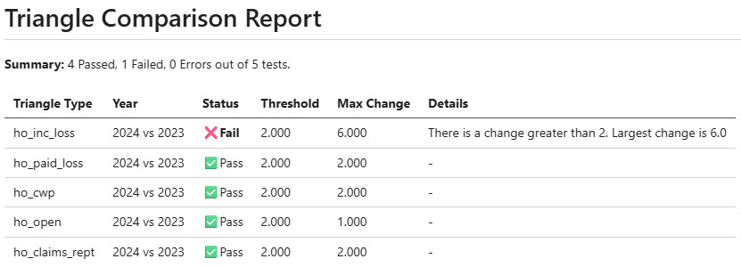
Historical recorded values should generally be unchanged in subsequent reports, assuming a consistent valuation date was used to determine development periods. In general, this does appear to be true in Tables 3 and 4, but there are still occasional differences, perhaps due to a very rare data restatement. If one accepts that small differences are “business as usual” based on past data, this pattern can be used to define a threshold beyond which a difference would be more alarming—perhaps beyond $10,000. The specific thresholds will require actuarial judgment. A failed check would not prove that something is wrong, but it should still be reviewed. Therefore, instead of immediately throwing an error and terminating the rest of the process, these types of conditions should be logged in a validation report. An analyst would be able to review the report once the pipeline completes and consider the highlighted issues holistically. Triangle_comparison.ipynb provides a more complete code example comparing several Schedule P triangles. A screenshot of the generated markdown report is shown in Figure 1, using arbitrary thresholds of $2,000 for losses and 2 for claim counts.

The results in this case are negligible, but a comparison between accident quarters is more likely to have larger differences. In addition to a threshold-based check, there are myriad other creative checks that could be useful. A test could flag if more than half the cells have changed or if the total absolute differences at a claim level reach a certain level.

Validation reports are not just for comparing against prior runs. These checks can also be used to compare against other sources of truth. For example, a team might like to confirm that the sum of the total paid claims in loss triangles reconciles against the general ledger. Logging metrics over time and generating a validation report primarily support accuracy and consistency.

The validation checks discussed above fall into two categories. The first type of embedded check, addressed in Section 4.2, throws an immediate error and halts the process, prompting the user to review the issue before either continuing the process or going back and fixing earlier processing steps. The second type of embedded check, discussed in Section 4.3, may log a potential issue but will still allow the remaining steps in the process to continue executing. The “warnings” would then be summarized in a report, as seen in Figure 1. Table 6 provides guidelines on when to use errors and warnings.

4.4. Maximize automation

The preceding discussion has reviewed numerous validation checks that could be performed on the input data, across the data pipeline, and on the final data product. To complement this process, another open-source tool specifically designed for data validation is helpful.

Pandera is a Python package that assists with data validation in Python-based data science pipelines. It features an expressive application programming interface (API) that offers sophisticated functionality out of the box while remaining flexible enough to customize.

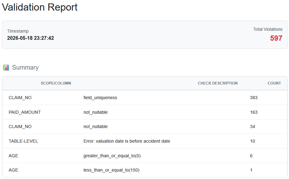
Pandera allows a user to define a basic “schema” to set expectations for a dataset’s behavior. For example, the following code will check the specified columns and ensure that the types and possible ranges of values match. It will check for inappropriately missing values and ensure uniqueness if specified. The penultimate check ensures that the accident date precedes a valuation date. The final check ensures that data is not accidentally omitted, as it would be strange for this insurer to not have any change in losses over a month.

claims_schema = pa.DataFrameSchema(
{
        'CLAIM_NO': pa.Column(str, unique=True, nullable=False),
        'AGE': pa.Column(float, checks=[pa.Check.ge(0), pa.Check.le(150)], 
nullable=True),
        'VALUATION_DATE': pa.Column(pa.DateTime, nullable=False),
        'DATE_OF_ACCIDENT': pa.Column(pa.DateTime, nullable=False),
        'PAID_AMOUNT': pa.Column(float, checks=[pa.Check.ge(0), 
pa.Check.le(1_000_000)], nullable=False)
    },
    checks = [
        pa.Check(
            lambda df: df['VALUATION_DATE'] >= df['DATE_OF_ACCIDENT'],
            name='valuation date should be after accident date',
            error='There are valuation dates prior to accident date'
        ),
        pa.Check(
            lambda df: 
df.groupby(df['VALUATION_DATE'].dt.to_period('M'))['PAID_AMOUNT'].sum().gt(0)
.all(),
            name='no_zero_loss_valuation_months',
            error='There are valuation months for which there are no losses!'
        ),
    ]
)

Pandera’s design makes it a superior choice for many validation checks compared to the custom code displayed in Sections 4.2 and 4.3. It allows users to designate a check as critical (and thus halt execution immediately) or minor (if investigation can wait until the entire process runs). It offers hypothesis testing for advanced reasonability checks. The syntax also makes it more approachable for new users and promotes consistency across the validation checks themselves.

Most importantly, schemas specified through pandera are reusable throughout the pipeline, meaning that the same “validate_data(df, claims_schema)” command can be executed every time the dataset is transformed. This allows a user to confirm, for example, that fields such as claim numbers remain unique through every step or that null values are never introduced into the accident date field.

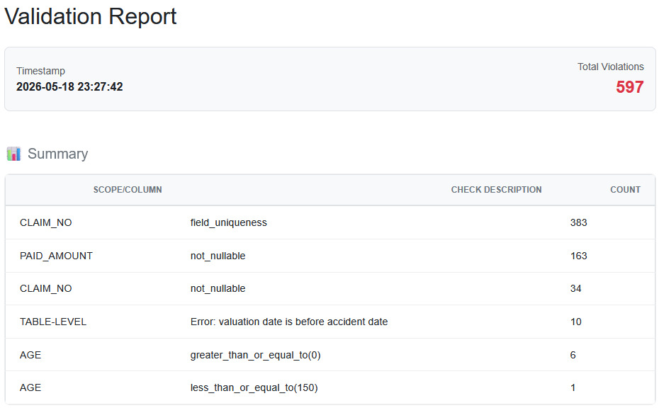
The results of the schema validation can be collected and displayed in a report once the pipeline finishes running. A more detailed example is available in pandera_validation.ipynb. The summary report shown in Figure 2 is generated as an HTML file.

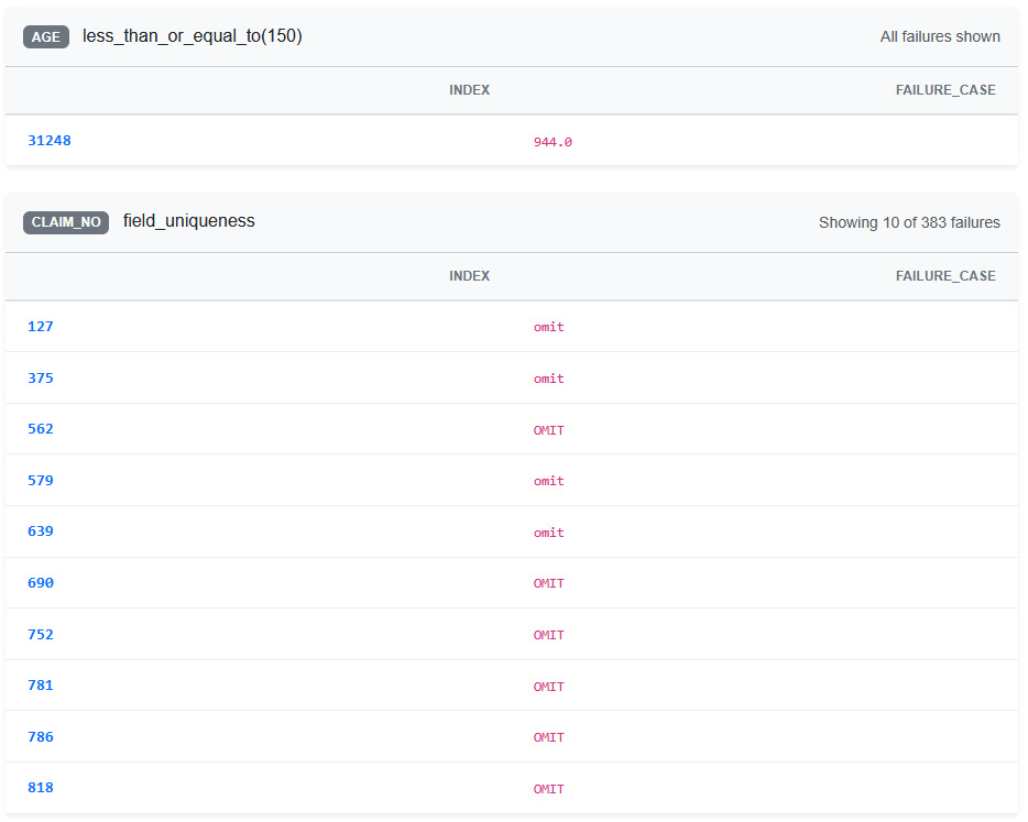
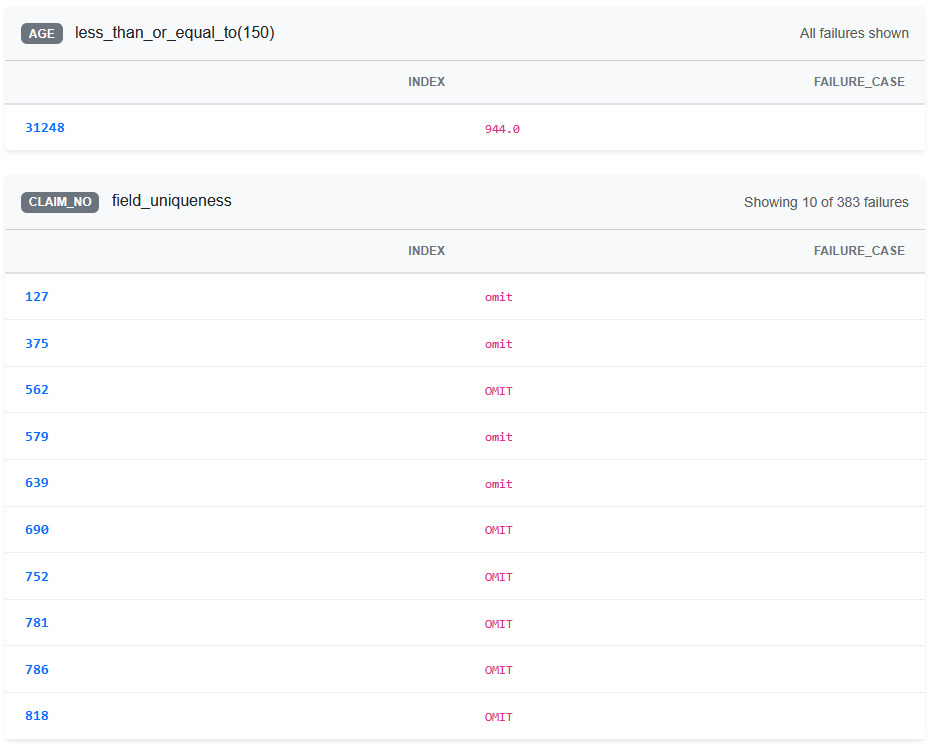
The report also includes details on failure cases for each check (Figure 3).

4.5. Plan for extensibility

The final best practice is to design the data pipeline in such a way that it can be easily extended. This could involve a joint planning session for upstream data teams and business users to discuss aspirational feature enhancements, untapped data sources, and new technologies. For new feature requests, there should be a mechanism for business users to sign off on the product prototyped by the data engineering team. This creates a perfect opportunity to determine an appropriate set of validation criteria for the updated pipeline.

The goal is to ensure that future maintenance work is well defined and that any new processes are consistent with established best practices. One example of a best practice with respect to data quality is to agree upon and regularly review current standards for validation checks in existing and new components. The embedded validation types discussed above can be encoded as templates to be reused for new transformation steps. All stakeholders should periodically review validation reports together. When there are multiple reserving teams with independent data pipelines, teams should discuss the differences to best leverage what can be borrowed across the organization. Thorough documentation specifying how to use and update these reports will also serve to onboard new coworkers.

As mentioned above, there can be trade-offs to calculating and manually reviewing some metrics, so a cost-benefit analysis may help to determine which checks are now obsolete and where blind spots remain. Actuarial Standard of Practice No. 23, Data Quality (Actuarial Standards Board 2016), states that an actuary should review the data for its suitability for an intended purpose. Therefore, they should prioritize developing checks for the fields that will be immediately used in an analysis over any supplementary information provided.

Two other major sources of data headaches are data integrations (e.g., due to a company acquisition) and platform migrations. Integrating data from another company is a massively complicated and potentially error-prone process. There is no silver bullet in this situation, but a common solution to ease the transition is to start with aligning data dictionaries. Recalling the consistency dimension of data quality, there should be a dedicated effort to canonicalize shared fields wherever possible. As with data validation checks, resolving incompatibilities as close to the data sources as possible can avoid much pain when tracing issues backward. From there, teams should agree on a go-forward data pipeline to use. Of course, this is easier said than done, and teams should keep in mind other considerations, such as the need to run two independent reserving processes in parallel during the transition. One issue that can be much harder to reconcile involves data freshness. Perhaps one source system refreshes its policy and loss data once a day, whereas another source system provides near real-time data. Depending on when the reserving data is pulled at the end of the month, there could be timing differences in the extracts that introduce rare inconsistencies.

A platform migration can be another fairly intensive effort. It requires collaboration from multiple business partners and raises many concerns: implementation responsibilities, project timelines, system validation procedures, onboarding, etc. The risk, as it relates to data quality, is that a new platform, language, or upgrade might change existing behavior unexpectedly. There are many different relational database management systems that support SQL, but the dialects will rarely differ from each other. One impactful difference is SAS’s PROC SQL, which is one of the only implementations that will permit an aggregation query in which not all of the non-aggregated select columns are in the “group by” clause. The following example will run successfully in SAS and will return a record for every claim ID, even though there is a chance that the user left the claim ID field in the select statement by mistake. Most other SQL databases would reject the query as invalid.

PROC SQL; SELECT lob, claim_id, SUM(paid_loss) FROM claims GROUP BY 1; QUIT;

It is often infeasible to learn about all the quirks of a new platform before rewriting processes. Creating small unit tests to confirm expected behavior can help pinpoint differences and prevent hard-to-debug surprises later.

5. Conclusion

Investigating data issues is an essential and often time-consuming process for reserving teams. Given the importance of data for regulatory compliance and the tight turnarounds required, reserving teams should take the opportunity to modernize and harden their processes. This paper discusses some new tools that can support this modernization effort, but the general principles outlined here can easily apply to any current workflow. Not all of these enhancements need to be adopted all at once—starting with just the smaller tasks will still pay dividends in the future. With that said, the greatest benefits will be realized by designing specific tests for each pipeline. The components that are most at risk of failing can differ radically across processes. The team’s data engineers and business users will be best equipped to address this by noting past failures and inefficiencies together.

In addition to data quality, the principles outlined in this paper will indirectly support other modernization initiatives. Including additional detail in data dictionaries can improve data discoverability across an organization. Setting up a centralized version control system may make it easier to safely integrate tools into a workflow. And agreeing upon clear standards for data pipelines eases communication between teams and shortens the turnaround time for incorporating new types of data and systems integrations.

---

Acknowledgments

This work was submitted to the 2026 Reserves Call Paper Program. The author is grateful for the support of the Reserves Working Group in publishing this paper. The views expressed in the paper are those of the author and do not necessarily reflect the views of his employer. The original datasets used are publicly available at the links listed below. These datasets may have been modified or adjusted before use in code examples to better demonstrate realistic data quality issues and concepts. They are used solely for illustrative purposes and should not be relied upon for other insights.

Data availability:

• https://www.kaggle.com/datasets/jhasony/privateinsurancedata/data

• https://www.kaggle.com/datasets/mustakimkureshi/dataset-car-insurance-claim/data

• https://data.mendeley.com/datasets/992mh7dk9y/2

Further reading

Actuarial Standards Board. 2016, December. Data Quality. ASOP 23. https://www.actuarialstandardsboard.org/asops/data-quality/.

DAMA International. 2017. DAMA-DMBOK: Data Management Body of Knowledge. 2nd ed. Technics Publications. https://technicspub.com/dmbok2/.

Hall, Graham, Mark Jones, Kevin Madigan, and Steve Zheng. 2020. Data Quality Management in the P&C Insurance Sector. Casualty Actuarial Society. https://www.casact.org/monograph/cas-monograph-no-9.