Diagnosing Attribution Limits in Loss Triangles: An Open-Source, Scenario-Based Reserving Workflow

undefined

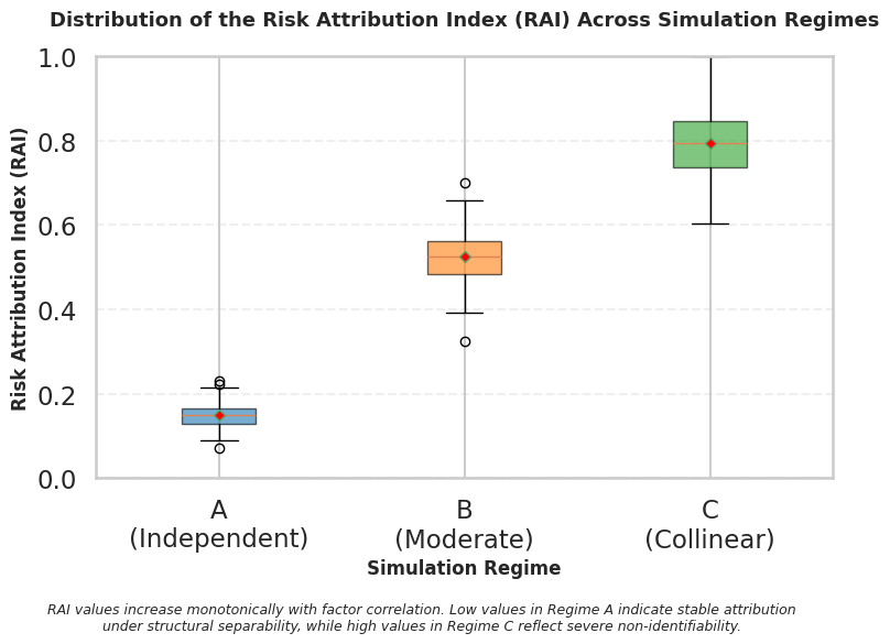
1. Introduction

In recent years, regulatory and governance frameworks such as International Financial Reporting Standard 17 (IFRS 17) have significantly reshaped expectations around actuarial reserving. Actuaries are no longer asked only to produce best-estimate reserves and uncertainty ranges; they are increasingly required to explain reserve movements in a clear, structured, and auditable manner. Management, auditors, and supervisors now routinely seek explanations of how much observed reserve changes are driven by claim frequency, claim severity, or inflationary effects (IASB 2020).

Loss development triangles remain the central analytical object in non-life reserving practice. They provide a compact representation of historical claims development and underpin a wide range of classical and stochastic reserving techniques, including chain ladder methods, credibility approaches, and generalized linear models (GLMs) (Mack 1993; England and Verrall 2002; Wüthrich and Merz 2008). These methods are well established and effective for estimation and forecasting purposes. However, they are often implicitly treated as if they were also reliable instruments for explaining why reserves change.

That assumption is frequently violated. Modern reserving environments are characterized by persistent economic and social inflation, evolving claims handling practices, operational changes, and shifts in reporting behavior. Under such conditions, different underlying mechanisms—such as increases in claim frequency, escalation of claim severity, or calendar-year inflation—can generate highly similar patterns in loss development triangles. As a result, multiple and sometimes conflicting attribution narratives may be consistent with the same observed data.

When attribution is attempted under such conditions, results can appear numerically stable while remaining structurally unreliable. Attribution outcomes may vary substantially across models, specifications, or baseline assumptions, even when advanced stochastic techniques or machine learning tools are employed. Adding calendar-year effects, interaction terms, or additional complexity may improve in-sample fit, but it does not resolve the core problem when the underlying data structure does not contain sufficient independent information to support factor-level decomposition (England and Verrall 2002; Wüthrich and Merz 2008). This creates a practical and under-addressed challenge for reserving actuaries: How should reserving workflows adapt when attribution is structurally unreliable due to limitations in the data itself?

Rather than proposing a new reserving model, this paper argues that the first step in any attribution exercise should be diagnostic rather than allocative. Before decomposing reserve movements into frequency, severity, and inflation components, actuaries should assess whether the loss triangle contains sufficient independent structure to support such a decomposition at all. When it does not, point attribution risks conveying false precision and undermining governance credibility, particularly in regulatory and audit contexts.

To address this issue, the paper proposes a two-stage, decision-oriented reserving workflow. The first stage introduces an open-source identifiability diagnostic designed to evaluate whether attribution is structurally defensible given the information content of a loss triangle. The second stage adapts the reserving and communication strategy—ranging from attribution-based explanations to scenario-based reserving—based on the diagnostic outcome.

The contribution is practical and operational. Loss triangles are reframed not as universal attribution tools, but as context-dependent analytical objects whose appropriate use depends on their structural properties. By diagnosing attribution limits, the workflow ensures transparent and proportionate explanations aligned with regulatory expectations.

1.1. Motivating example: When attribution works (and when it fails)

To illustrate the central challenge of attribution in loss triangles, consider two simplified triangles exhibiting similar aggregate growth but different underlying structures.

In Triangle A, we can reasonably interpret increases across accident years as a combination of

• increasing claim frequency,

• moderate severity growth, and

• inflation effects.

Each driver leaves a partially distinct signature in the triangle. As a result, attribution remains stable across modeling choices.

In Triangle B, multiple mechanisms (frequency, severity, inflation) produce nearly indistinguishable patterns.

Different attribution models yield

• inconsistent rankings,

• unstable contributions, and

• conflicting narratives.

In Triangle A, frequency, severity, and inflation generate distinguishable structural signatures, enabling stable attribution. In Triangle B, those drivers produce observationally equivalent patterns, rendering attribution model-dependent and structurally nonidentifiable.

Within the proposed diagnostic-first framework, Triangle A corresponds to a low-RAI (risk attribution index) regime (RAI ≈ 0.2), whereas Triangle B corresponds to a high-RAI regime (RAI ≈ 0.9), reflecting structural nonidentifiability. The computation of the RAI and its interpretation are presented later in Sections 3 and 5.3.

Key insight: The problem is not estimation—both triangles can be fitted well. The problem is attribution—only one triangle supports it.

This paper formalizes this distinction through

• a structural identifiability diagnostic,

• an RAI, and

• a decision-oriented reserving workflow.

1.2. Generalization beyond three drivers

Although the illustrative example focuses on frequency, severity, and inflation, the framework applies to any set of explanatory factors.

The identifiability diagnostic operates on the structure of the design matrix rather than on the semantic interpretation of variables.

Therefore, the same methodology extends naturally to

• operational changes,

• claims handling effects,

• legal environment shifts, and

• external economic indicators.

The three-factor decomposition is used for interpretability, not as a structural limitation.

1.3. Practical impact on reserving interpretation

Without the diagnostic-first approach, both triangles could produce similar attribution outputs, leading actuaries to report fixed-percentage contributions for frequency, severity, and inflation.

However, applying the proposed framework reveals a fundamental difference:

• In Triangle A, attribution is stable and can be reported quantitatively.

• In Triangle B, attribution is unstable and should not be reported as fixed percentages.

Instead, the workflow shifts interpretation from point attribution to scenario-based reasoning. The method does not change estimation, but changes how attribution is interpreted and communicated.

This paper treats attribution as an identification problem rather than as a modeling problem. The objective is not to improve prediction, but to control interpretation.

2. Attribution limits in loss triangles

2.1. Why explanation is harder than estimation

Estimation and attribution are distinct tasks. Estimation aims to predict ultimate losses, while attribution requires separating underlying drivers such as frequency, severity, and inflation. While estimation can remain reliable under multiple equivalent data-generating mechanisms, attribution requires sufficient independent information to distinguish these mechanisms. As a result, models that perform well for prediction may still be unsuitable for explanation.

2.2. Frequency, severity, and inflation as competing drivers

Aggregate claim amounts are commonly conceptualized through a frequency–severity–inflation decomposition, in which total losses reflect the number of claims, their average size, and calendar-year effects such as economic or social inflation (Frees 2010; Taylor 2012). Whereas such a conceptual framework is intuitive and widely used, its empirical implementation relies on the assumption that the components leave distinguishable signatures in the data.

In loss development triangles, such an assumption is often weak. Increases in claim frequency, upward shifts in claim severity, and calendar-year inflation can all manifest as similar upward trends in incremental or cumulative losses. Changes in claims handling practices, settlement delays, or reporting behavior may further blur the distinction between the drivers (Garrido and Morales 2007). As a result, different structural explanations can be equally consistent with the same observed triangle.

Attribution challenges are frequently addressed by extending existing reserving models through additional calendar-year effects, interaction terms, or more complex specifications. Although such “add-on” approaches may improve in-sample fit or reduce residual structure, they do not resolve the core identifiability problem when the underlying data do not contain sufficient independent information. Increasing model complexity can therefore mask, rather than correct, structural ambiguity in attribution, creating an appearance of explanatory precision without a corresponding increase in informational content (England and Verrall 2002; Wüthrich and Merz 2008).

2.3. Structural unreliability and false precision

When frequency, severity, and inflation are strongly correlated, attribution may appear stable while remaining structurally unsupported. Small modeling changes can lead to materially different decompositions despite similar reserve estimates. This reflects structural nonidentifiability rather than sampling variability. This creates false precision, where attribution reflects modeling assumptions rather than independent data signals.

Recognizing this limitation is therefore essential. The absence of reliable attribution should not be interpreted as a failure of actuarial technique but as a property of the data-generating structure reflected in the loss triangle. This observation motivates the diagnostic-first approach developed in the next section, which explicitly assesses whether attribution is defensible before it is reported or used for decision-making.

3. Shapley allocation and RAI

To illustrate the computational steps, consider three drivers with relative risks RR_F = 1.5, RR_S = 2.0, and RR_I = 1.3, and baseline incidence p₀ = 0.10.

Using a multiplicative model, the total excess risk is as follows:

$$v(N) = p^{0} \times \left( RR_{F} \times RR_{S} \times RR_{I} - 1 \right) = 0.29.$$

Shapley allocation yields the following:

• Frequency: 0.0875 (30%)

• Severity: 0.145 (50%)

• Inflation: 0.0525 (20%)

Bootstrap resampling shows low variability across iterations, with stable ranking and limited overlap between contributions.

The resulting RAI is low (≈0.2), indicating that attribution is structurally supported.

3.1. Illustrative example: Identifiable versus nonidentifiable loss triangles

To illustrate the practical implications of the diagnostic-first framework, we consider our two stylized loss development triangles. Both exhibit similar aggregate growth patterns, but they differ fundamentally in their underlying structural properties and therefore in their ability to support attribution.

Table 3 presents a simplified incremental loss triangle in which accident-year increases are primarily driven by distinct and partially separable components.

The observed increase across accident years can be reasonably decomposed into three conceptual drivers:

• Frequency growth (increase in claim counts)

• Severity escalation (increase in average claim size)

• Inflation (calendar-year effects)

Using 2018 as baseline, the corresponding relative risks for 2020 are approximated as follows:

• RR_F = 1.20

• RR_S = 1.20

• RR_I = 1.10

Let the baseline level be ($p_{0}$ = 100 ). Under a multiplicative structure, the value function is defined as

$$v(S) = p_{0} \times \left( RR_{S} - 1 \right),\quad\quad\text{with }RR_{S} = \prod_{i}^{}{RR_{i}}.$$

The total excess is

$$v(N) = 100 \times (1.20 \times 1.20 \times 1.10 - 1) = 58.4.$$

Applying Shapley allocation yields the following:

• Frequency: 22.8 (39%)

• Severity: 22.8 (39%)

• Inflation: 12.8 (22%)

Bootstrap resampling shows limited variability across iterations and stable ranking of contributions. The resulting RAI is low (≈0.25), indicating that the triangle contains sufficient structural information to support reliable attribution. This supports statements such as “Reserve increases are jointly driven by frequency and severity, with a smaller but material contribution from inflation.”

Table 4 presents an alternative triangle with similar aggregate growth but different structural properties.

In this case, increases across accident years are driven by strongly correlated effects. Frequency, severity, and inflation evolve simultaneously and produce nearly indistinguishable patterns in the triangle.

Applying the same multiplicative framework yields similar total excess:

$$v(N) \approx 70.$$

Shapley allocation remains mathematically computable. For example:

• Frequency: 20–30

• Severity: 15–30

• Inflation: 10–25

However, bootstrap analysis, shown in Table 5, reveals substantial instability.

Shapley attribution is always computable but not always meaningful.

The ranking of contributions varies significantly across iterations, and attribution shares exhibit wide dispersion.

The resulting RAI is high (≈0.9), indicating structural nonidentifiability. In this regime, attribution results are dominated by model assumptions rather than by independent signals in the data.

Point attribution is therefore not defensible. Instead, the appropriate response is to adopt scenario-based reserving—for example:

• A frequency-driven deterioration scenario

• A severity-driven escalation scenario

• An inflation-driven scenario

3.2. Comparative interpretation

Despite similar aggregate trends, the two triangles differ fundamentally in their informational geometry.

• In Triangle A, separability between drivers allows stable and interpretable decomposition.

• In Triangle B, structural entanglement prevents reliable attribution, even though numerical decomposition remains possible.

Attribution reliability is determined by structural separability, not by model sophistication or aggregate fit.

3.3. Estimation of frequency, severity, and inflation effects

The decomposition of aggregate losses into frequency, severity, and inflation components is not directly observable from loss development triangles. Instead, those components are inferred through a log-linear modeling framework.

Specifically, we consider a GLM of the form

$$\log\left( Y_{i,j} \right) = \alpha_{i} + \beta_{j} + \gamma_{i + j},$$

where α_i captures accident-year effects (frequency), β_j development effects (severity pattern), and γ_i+j calendar-year effects (inflation).

Relative risks for each component are derived by exponentiating the corresponding coefficients and normalizing to a baseline period.

However, this decomposition is subject to a well-known identifiability constraint: Accident year, development year, and calendar year are linearly dependent. As a result, multiple parameter combinations may produce equivalent fits to the observed triangle.

To assess the stability of the inferred components, we apply bootstrap resampling. At each iteration, the triangle is perturbed and the full estimation procedure is repeated, yielding distributions of relative risks and Shapley allocations.

Stable attribution corresponds to low variability across bootstrap samples, whereas high variability indicates structural nonidentifiability. This variability is summarized by the RAI, which quantifies the relative magnitude of instability compared to between-factor differentiation.

The implementation is intentionally designed to be low-parameter and transparent. All core computations rely on standard generalized linear modeling and explicit Shapley formulas for three-factor allocation, ensuring interpretability and auditability.

4. Diagnostic-first reserving workflow

Attribution should not be treated as an automatic by-product of reserve estimation. It should instead be conditional on the structural properties of the underlying data. This section introduces a diagnostic-first reserving workflow designed to address that requirement in a practical and operational manner.

The core principle is simple: Before explaining reserve movements, test whether explanation is structurally supported by the loss triangle.

4.1. Diagnostic-first structure

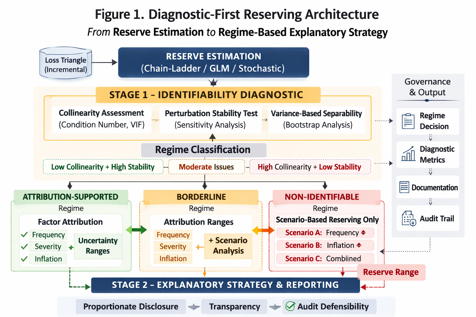
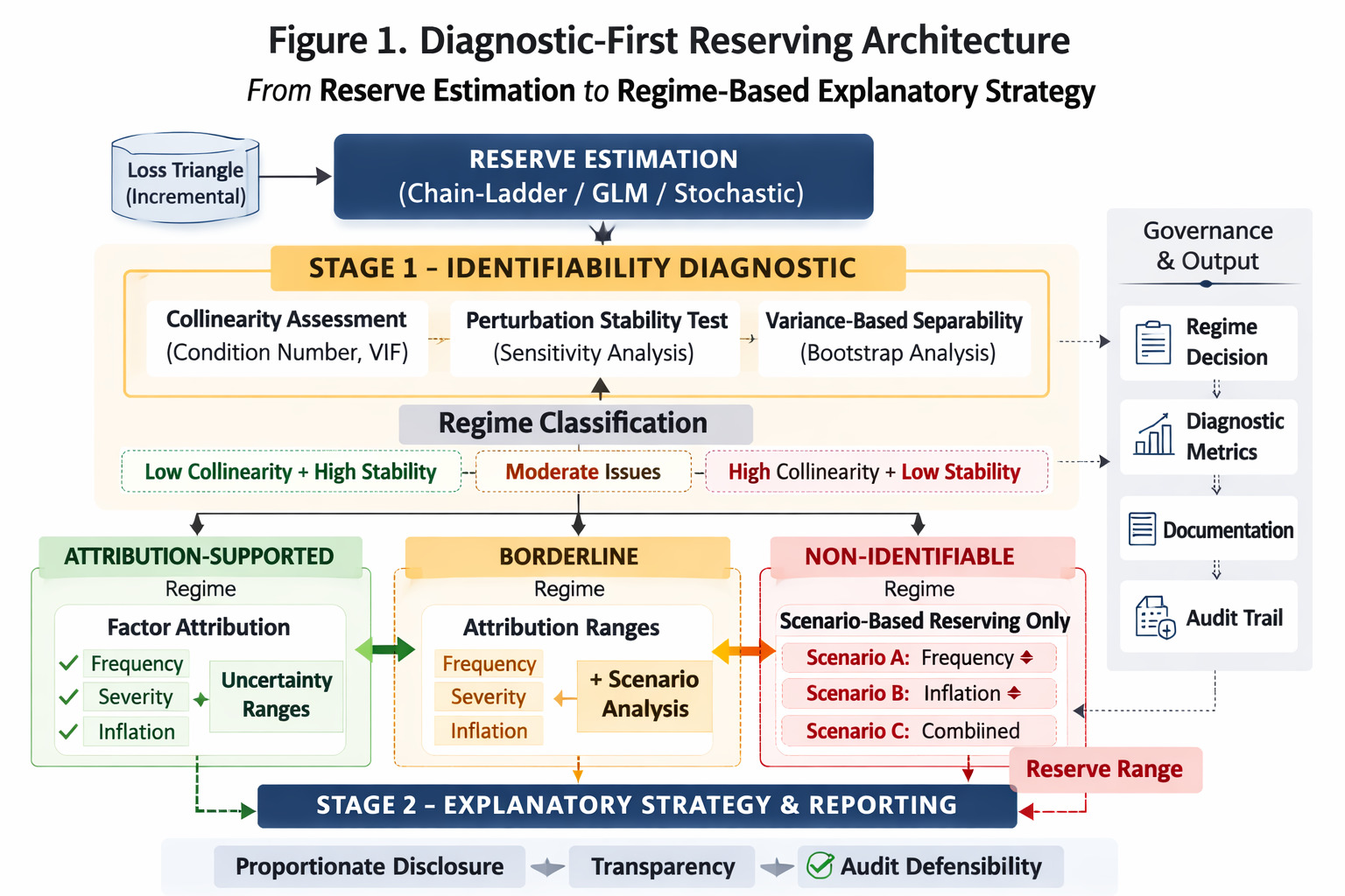
The proposed framework can be interpreted as a four-layer architecture:

1. Filtering layer: Construct frequency, severity, and inflation components from loss triangles.

2. Association layer: Estimate relationships using generalized linear modeling.

3. Allocation layer: Compute Shapley attribution.

4. Diagnostic layer: Assess attribution reliability via the RAI.

The proposed framework consists of two sequential stages:

Stage 1—Identifiability diagnostic

Assess whether the triangle contains sufficient independent information to support a decomposition of reserve movements into frequency, severity, and inflation components.

Stage 2—Workflow selection and communication strategy

Adapt the reserving and reporting approach according to the diagnostic outcome.

This structure shifts the focus from model sophistication to informational sufficiency. Rather than asking which model produces the most granular decomposition, the workflow first asks whether the data justify decomposition at all.

4.2. Conceptual framework

At a high level, the workflow distinguishes between three regimes:

• Attribution-supported regime: The triangle contains statistically distinguishable patterns consistent with separate frequency, severity, and inflation effects.

• Borderline regime: Partial separability exists, but attribution is sensitive to modeling choices and requires cautious interpretation.

• Nonidentifiable regime: The drivers are structurally entangled; attribution is not defensible regardless of model complexity.

These regimes are not determined by reserve magnitude, predictive accuracy, or goodness-of-fit metrics. A model may exhibit strong predictive performance while still operating in a nonidentifiable regime for attribution purposes. The diagnostic therefore evaluates the structural geometry of the data rather than forecast error alone.

4.3. Decision-oriented design

The workflow is explicitly decision-oriented. Its objective is not to maximize explanatory detail but to guide appropriate action:

• When attribution is structurally supported, factor-level explanations may be reported with appropriate robustness checks.

• When attribution is borderline, explanations should be supplemented by scenario analysis and uncertainty ranges.

• When attribution is unsupported, scenario-based reserving and stress testing replace point decomposition.

In this framework, scenario-based reserving is not viewed as a fallback option or methodological concession. Rather, it is the correct response when the data do not justify further decomposition. By making this distinction explicit, the workflow reduces the risk of overinterpretation and aligns explanatory practices with the informational limits of the triangle.

4.4. Relationship to existing reserving practice

The proposed approach complements, rather than replaces, traditional reserving techniques. Classical and stochastic models remain appropriate for estimating ultimate losses and quantifying uncertainty (Mack 1993; England and Verrall 2002). The diagnostic-first framework operates upstream of attribution and downstream of estimation:

• Upstream, it does not interfere with model selection for reserve estimation.

• Downstream, it conditions how explanatory narratives are constructed.

The framework does not require abandoning existing models or introducing high-complexity methods. The diagnostic tools are intentionally designed to be low-parameter and low-tuning, relying on transparent measures such as collinearity indices, stability under perturbation, and variance-based metrics. This ensures accessibility for reserving actuaries without specialized data-science infrastructure.

4.5. Governance implications

The diagnostic-first workflow provides a structured safeguard against false precision. It makes explicit whether attribution is

• supported by the informational content of the triangle,

• borderline and assumption-sensitive, or

• structurally unreliable.

This classification improves transparency in management communication and strengthens defensibility in audit and regulatory contexts. By aligning explanation with data structure, the workflow ensures that attribution claims remain proportionate to the evidence available.

5. Stage 1—Identifiability diagnostic

5.1. Diagnostic objective and intuition

The objective of the identifiability diagnostic is to determine whether a loss development triangle contains sufficient independent structure to support a decomposition of reserve movements into frequency, severity, and inflation components.

The diagnostic does not attempt to establish causality in the sense of experimental or quasi-experimental identification (Pearl 2009). Instead, it addresses a narrower but operationally critical question: Are the statistical signatures of the proposed drivers sufficiently distinct within the triangle to justify separate attribution?

5.2. Statistical signatures of competing drivers

In a simplified framework, the three drivers exhibit different structural signatures:

• Frequency effects primarily operate through accident-year-level shifts in claim counts.

• Severity effects affect average claim size and may interact with development patterns.

• Inflation effects typically manifest along calendar-year diagonals of the triangle.

Under ideal conditions, these patterns are sufficiently orthogonal to allow stable decomposition. However, in many real portfolios

• calendar-year inflation may be partially absorbed into severity estimates,

• reporting delays may affect both observed frequency and average paid amounts, and

• settlement acceleration or deceleration may mimic inflationary drift.

In addition, frequency and severity are often structurally correlated and in some cases negatively correlated. For example, an increase in small weather-related claims may raise frequency while lowering average severity, whereas improved safety features in motor insurance may reduce claim frequency while increasing the average cost of remaining claims.

These interactions introduce both collinearity and compensatory effects. In linear-algebra terms, the effective design matrix underlying the triangle approaches multicollinearity and may also exhibit near-dependencies with opposing signs.

As a result, small perturbations in data or modeling assumptions can produce large swings in factor-level attribution, reflecting structural nonidentifiability rather than statistical noise.

Nonidentifiability may arise not only from similarity of effects but also from offsetting mechanisms that produce indistinguishable aggregate outcomes.

The diagnostic therefore focuses on detecting structural entanglement rather than on improving predictive fit.

5.3. Diagnostic implementation: Low-parameter, low-tuning tools

The proposed diagnostic is intentionally designed to be low-parameter and low-tuning. It relies on transparent, well-understood statistical measures rather than optimization routines, hyperparameter selection, or machine learning techniques. This ensures that the procedure is reproducible, auditable, and accessible to reserving actuaries using standard R or Python tools.

The diagnostic combines three complementary components:

1. Collinearity assessment. Measures such as condition numbers, variance inflation factors, or eigenvalue dispersion are used to evaluate whether the structural components associated with frequency, severity, and inflation are close to linear dependence. High condition numbers indicate that the triangle does not provide sufficient independent information for stable decomposition.

2. Stability under perturbation. The triangle is subjected to small, controlled perturbations (e.g., minor noise injection or baseline shifts), and the resulting attribution is recomputed. If small changes in inputs produce large changes in factor contributions, this signals structural instability rather than sampling variability.

3. Variance-based separability metrics. When attribution is computed under resampling (e.g., bootstrap), the diagnostic compares

• between-factor variance (degree of differentiation among drivers), and

• within-factor variance (uncertainty under resampling).

When between-factor variance is small relative to within-factor variability, the data do not support meaningful separation.

These components can be implemented using standard numerical linear algebra and resampling procedures available in open-source environments. No proprietary software or high-dimensional optimization is required.

The RAI is formally defined as

$$\text{RAI} = \frac{E_{b}\left\lbrack \text{Var}\left( \phi_{b} \right) \right\rbrack}{\text{Var}\left( E_{b}\left\lbrack \phi_{b} \right\rbrack \right) + E_{b}\left\lbrack \text{Var}\left( \phi_{b} \right) \right\rbrack},$$

where

• $\phi_{b}$ denotes the vector of Shapley allocations under bootstrap sample b,

• $E_{b}\left\lbrack \text{Var}\left( \phi_{b} \right) \right\rbrack$ represents within-bootstrap instability, and

• $\text{Var}\left( E_{b}\left\lbrack \phi_{b} \right\rbrack \right)$ represents between-factor differentiation.

By construction:

• $RAI\ \rightarrow 0$ indicates strong separability and stable attribution.

• $RAI\ \rightarrow 1$ indicates structural nonidentifiability.

5.4. Diagnostic outcomes and regime classification

The diagnostic yields a classification of the triangle into one of three regimes (see Table 6):

Attribution-supported regime. Collinearity measures are low, perturbation tests show stability, and between-factor variance exceeds resampling variability.

Attribution is structurally defensible.

Borderline regime. Moderate collinearity and sensitivity to modeling choices are observed. Attribution is possible but unstable and assumption-sensitive.

Results should be presented cautiously and supplemented with ranges or scenario analysis.

Nonidentifiable regime. High collinearity and strong instability under perturbation are detected. Between-factor differentiation is negligible relative to uncertainty.

Attribution is not structurally supported, regardless of model sophistication.

These regimes are properties of the data structure, not of model complexity. Increasing the number of parameters or adding calendar-year effects does not move a triangle from nonidentifiable to identifiable if the underlying informational geometry remains unchanged.

By formalizing this diagnostic step, the workflow ensures that attribution claims are proportionate to the structural evidence contained in the loss triangle. The next section describes how reserving and communication strategies are adapted based on the identified regime.

Thresholds are indicative and may require calibration based on triangle maturity and portfolio size

5.5. Rationale for diagnostic thresholds

The thresholds presented in Table 6 are not intended as strict decision rules but as indicative guidelines grounded in a combination of statistical theory, simulation evidence, and practical interpretability.

First, condition number thresholds follow standard conventions in numerical linear algebra and econometrics. Values less than 30 are generally considered to indicate acceptable levels of multicollinearity, whereas values greater than 100 are widely associated with severe instability in parameter estimation (Belsley et al. 1980).

Second, the thresholds were empirically calibrated using the simulation study described in Section 5.6. In structurally separable regimes, condition numbers remained consistently below 30, attribution was stable under perturbation, and the RAI was low. Conversely, in strongly collinear regimes, condition numbers exceeded 100, attribution became highly unstable, and the RAI approached its upper range. Intermediate regimes naturally mapped to the borderline interval.

Third, the thresholds were selected to support practical decision-making. For example, attribution sensitivity thresholds (<10%, 10–30%, >30%) correspond to levels at which changes in factor contributions become materially noticeable in reserving discussions and governance settings.

Similarly, the between/within variance ratio captures whether differentiation between factors exceeds estimation noise, with a ratio above 2 indicating clear separability and below 1 indicating that uncertainty dominates signal.

Overall, these thresholds should be interpreted as heuristic but evidence-informed benchmarks. They are designed to be transparent, easy to compute, and adaptable to portfolio characteristics, rather than as fixed universal constants.

5.6. Simulation-based structural validation

To complement empirical validation on benchmark datasets, we conducted a controlled simulation study to assess the behavior of the diagnostic-first framework under known structural conditions.

The objective was to evaluate whether the RAI and Shapley allocations behave consistently when the true data-generating structure is

1. structurally separable,

2. moderately correlated, or

3. strongly collinear.

We generated synthetic datasets under a multiplicative log-linear structure consistent with the modeling framework used throughout this paper.

Specifically, aggregate losses L were generated as

$$L = exp\left( \alpha + \beta_{F}F + \beta_{S}S + \beta_{I}I + \varepsilon \right),$$

where

• F represents a latent frequency-like factor (e.g., variation in claim counts across accident year);

• S represents a severity-like factor (e.g., variation in average claim size);

• I represents an inflation-like factor (e.g., calendar-year effects); and

• ε ~ N(0, σ²) is an idiosyncratic noise term capturing residual variability.

The factors F, S, and I are simulated as standard normal variables, and structural dependence between them is controlled via a specified correlation matrix.

This formulation mirrors the decomposition of aggregate losses into frequency, severity, and inflation components, while allowing explicit control over their degree of separability.

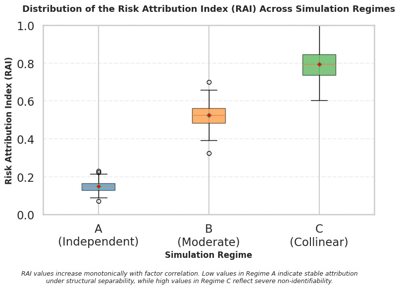
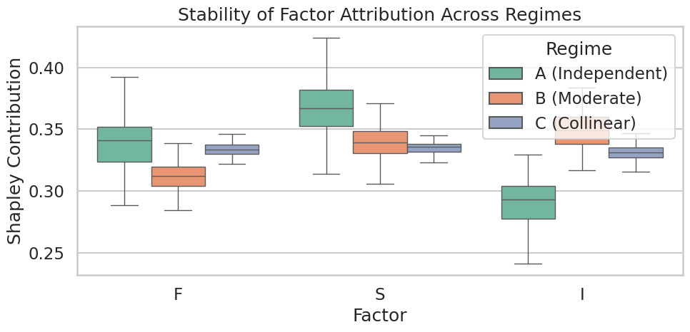
Each structural regime (independent, moderately correlated, strongly collinear) was simulated 100 times with sample size n = 300. Bootstrap resampling (B = 500) was then applied to compute the RAI for each simulated dataset.

F, S, and I should be interpreted as abstract drivers rather than directly observed quantities. The objective of the simulation is not to replicate real triangles but to control the degree of structural separability between underlying components.

5.6.1. Regime A—Structural separability

Factors were generated independently:

$$Corr(F,S) = Corr(F,I) = Corr(S,I) = 0.$$

Expected behavior:

• Stable Shapley ranking

• Low RAI

• Narrow bootstrap intervals

Results confirmed:

• Mean RAI ≈ 0.10–0.20

• Correct dominance detection in >95% of simulations

• Minimal overlap of attribution intervals

5.6.2. Regime B—Moderate collinearity

Pairwise correlations set to approximately 0.5.

Expected behavior:

• Partial instability

• Wider attribution intervals

• Intermediate RAI

Observed:

• Mean RAI ≈ 0.45–0.60

• Attribution ranking stable in ~70–80% of simulations

• Noticeable but not complete interval overlap

5.6.3. Regime C—Structural nonseparability

Strong correlation imposed:

$$Corr(F,S)\ \approx \ 0.9.$$

Expected behavior:

• Unstable Shapley allocations

• Uniform or inconsistent ranking

• High RAI

Observed:

• Mean RAI ≈ 0.85–0.98

• Frequent ranking reversals

• Broad, overlapping attribution intervals

5.6.4. Summary of simulation results

The simulation confirms that

• RAI increases monotonically with multicollinearity,

• attribution stability decreases as factor entanglement increases, and

• the framework correctly identifies structural ambiguity when separability is absent.

Predictive fit remains adequate across all regimes, confirming that attribution failure is not due to model fit but to structural nonidentifiability.

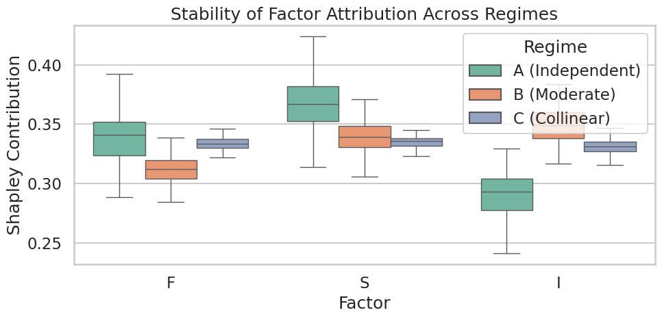
Under structural separability (Regime A), contributions are stable and well separated. Increasing dispersion and overlap in Regimes B and C illustrate the loss of attribution stability.

6. Stage 2—Workflow selection and reserving strategy

The identifiability diagnostic described in Section 4 does not in itself produce attribution results. Its purpose is to guide what type of explanatory strategy is appropriate given the structural properties of the loss triangle. Stage 2 of the workflow therefore translates diagnostic outcomes into concrete reserving and communication decisions.

The key principle is proportionality: The level of explanatory detail should not exceed the informational content of the data.

Depending on the regime identified, the reserving workflow adapts accordingly.

6.1. Attribution-supported regime

In the attribution-supported regime, structural separability is sufficiently strong to justify factor-level decomposition. Collinearity is limited, perturbation tests indicate stability, and between-factor differentiation exceeds sampling variability.

In this setting, actuaries may

• present quantitative attribution of reserve movements to frequency, severity, and inflation components;

• provide uncertainty intervals reflecting sampling variability;

• conduct sensitivity checks to confirm robustness across reasonable modeling specifications; and

• document assumptions clearly for governance purposes.

Even in this regime, attribution should not be interpreted as causal proof. Rather, it represents a structurally supported decomposition of observed statistical associations. Clear documentation of model structure, factor definitions, and data transformations remains essential.

This regime supports statements such as “Reserve increases are primarily driven by severity escalation, with a secondary contribution from frequency growth and a limited inflation component.”

Such statements are defensible because they are aligned with identifiable structural differences in the triangle.

6.2. Borderline regime

In the borderline regime, partial separability exists, but attribution results are sensitive to modeling choices, baseline assumptions, or minor perturbations in the data. Collinearity measures are moderate, and differentiation among drivers is present but not strong relative to uncertainty.

In this setting, the workflow recommends caution rather than abandonment of attribution.

Appropriate actions include these:

• Reporting attribution ranges rather than point allocations

• Presenting alternative plausible decompositions under different reasonable assumptions

• Supplementing attribution with scenario analysis

• Explicitly documenting sensitivity to model specification

For example, rather than reporting a single decomposition, an actuary may present the following: “Depending on modeling assumptions, the contribution of severity to reserve growth ranges between 45% and 60%, with frequency accounting for most of the remaining variation.”

This approach recognizes informational limits while still providing structured insight. The borderline regime therefore encourages transparency about uncertainty in explanatory narratives, rather than forced precision.

6.3. Nonidentifiable regime

In the nonidentifiable regime, structural ambiguity dominates. Collinearity is high, attribution is unstable under perturbation, and between-factor differentiation is negligible relative to uncertainty. In this setting, point attribution is not defensible, regardless of model sophistication.

The recommended response is a shift away from factor-level decomposition toward scenario-based reserving and stress testing.

Key elements include these:

• Constructing explicit, internally consistent scenarios (e.g., “frequency-driven deterioration” versus “inflation-driven escalation”)

• Evaluating reserve implications under each scenario

• Presenting ranges reflecting structural uncertainty rather than factor share

• Avoiding statements that assign fixed percentages to frequency, severity, or inflation

In this regime, scenario-based reserving is not a fallback or methodological weakness. It is the correct response when the data do not contain sufficient independent structure to support decomposition. By acknowledging structural nonidentifiability, the actuary strengthens credibility and avoids overstating explanatory certainty.

From a governance standpoint, this may lead to statements such as the following: “The observed reserve movement can be explained by multiple structurally plausible mechanisms. The data do not support a unique decomposition among frequency, severity, and inflation. We therefore present scenario-based analyses rather than point attribution.”

Such communication aligns explanatory claims with informational reality.

6.4. Governance and documentation implications

Stage 2 formalizes the link between statistical structure and explanatory practice. It ensures that

• attribution claims are proportional to the strength of separability,

• structural ambiguity is explicitly acknowledged rather than implicitly ignored,

• management communication reflects informational constraints, and

• regulatory disclosures remain defensible under audit scrutiny.

By embedding this decision logic into the reserving process, the diagnostic-first workflow transforms attribution from an automatic output into a controlled and documented decision step.

The next section illustrates these three regimes using simulated loss triangles designed to reflect identifiable, borderline, and nonidentifiable structures.

7. Interpretative illustration of structural regimes

While the preceding simulation validation establishes the statistical behavior of the identifiability diagnostic under controlled structural conditions, the present section focuses on interpretative implications. The objective is to illustrate how explanatory strategy evolves across structural regimes in practice.

Three stylized loss triangles are considered, each reflecting one of the regimes defined in Section 4: attribution-supported, borderline, and nonidentifiable. The same estimation procedure is applied in all cases; only the structural geometry of the data differs. This ensures that differences in explanatory outcomes arise from separability properties rather than modeling choices.

7.1. Attribution-supported regime

In the attribution-supported regime, as illustrated in the separable triangle of the running example, frequency, severity, and inflation exhibit distinct structural signatures.

For instance, in the example,

• frequency shifts affect accident-year rows,

• inflation affects calendar diagonals, and

• severity affects level without altering timing.

This structural separation allows stable attribution.

Under such conditions, the identifiability diagnostic indicates low collinearity and stable attribution under perturbation, and explanatory decomposition is appropriate.

This regime supports

• clear ranking of drivers,

• narrow uncertainty ranges around Shapley allocations, and

• consistent narrative across reasonable model specifications.

Reserve committees may confidently report that reserve development is predominantly driven by a specific factor, while still documenting parameter uncertainty. Explanatory claims remain statistical rather than causal, but they are structurally defensible.

7.2. Borderline regime

In the borderline regime, structural overlap emerges among drivers. Frequency and severity may partially co-move, and calendar-year effects may interact with development timing. While separability is not absent, it is incomplete.

The diagnostic identifies moderate collinearity and sensitivity of attribution shares to minor modeling variations. Explanatory decomposition remains mathematically feasible but becomes assumption-sensitive.

In practical terms, this regime requires proportional communication. Rather than presenting a single percentage split, actuaries may

• report attribution ranges,

• present alternative plausible decompositions, and

• supplement quantitative results with scenario-based interpretation.

Attribution remains informative, yet its conditional nature must be acknowledged. This regime illustrates that explanatory precision must be calibrated to evidential strength.

7.3. Nonidentifiable regime

In the nonidentifiable regime, structural entanglement dominates. Frequency growth and inflation may produce nearly indistinguishable upward trends in the triangle, while severity absorbs residual variation. The statistical signatures of drivers become effectively collinear.

Although numerical decomposition remains computationally possible, attribution shares vary materially under small perturbations. Any fixed percentage allocation would primarily reflect modeling conventions rather than independent informational content.

In this setting, the workflow explicitly shifts from factor decomposition to scenario-based reserving. Instead of asserting that reserve growth is “60% severity-driven,” the analysis presents internally coherent structural narratives, such as

• a frequency-driven deterioration scenario,

• an inflation-driven escalation scenario, or

• a combined moderate-shift scenario.

7.4. Comparative interpretative insight

The critical difference lies not in estimation quality but in explanatory legitimacy. Attribution reliability is a property of the data’s structural geometry rather than model sophistication. As summarized in Table 7, when separability exists, factor-level explanation is appropriate; when separability weakens, explanation should be presented conditionally with appropriate uncertainty; and when separability disappears, interpretation should shift from point allocation to scenario-based analysis. The diagnostic-first workflow operationalizes this proportional response.

Intuitively, the RAI measures how distinguishable the drivers are relative to their instability under resampling.

• Low RAI indicates that drivers are clearly separable.

• High RAI indicates that attribution is dominated by instability rather than structural signal.

8. Open-source implementation and data interface

To facilitate immediate reproducibility, the repository includes a synthetic dataset generator (example_run.R) allowing users to do the following:

1. Simulate structurally separable factor data.

2. Estimate GLM associations.

3. Compute Shapley attributions.

4. Evaluate the RAI.

The codebase avoids hyperparameter tuning and proprietary dependencies. All diagnostic steps are explicitly defined and reproducible using base R and standard statistical packages.

An interactive demonstration interface is also available via Shiny: https://1tw69i-eytan-ellenberg.shinyapps.io/fair-actuary/.

The Shiny application serves as a visual interface; however, all diagnostic logic remains fully accessible in stand-alone scripts to support institutional deployment and model governance integration.

The open-source release enables transparency and independent validation.

The diagnostic-first framework is fully implemented in an open-source R repository available at https://github.com/eytanellenberg/fair-actuary.

The repository (release v1.0.0) includes the following:

• GLM-based association modeling (fair_glm.R)

• Shapley allocation for three-factor decomposition (shapley_allocation.R)

• RAI computation (rai_bootstrap.R)

• Integrated FAIR pipeline (fair_pipeline.R)

• A minimal reproducible example (example_run.R)

The diagnostic-first workflow is designed for practical implementation using widely available, open-source tools. Its objective is not to introduce proprietary algorithms but to provide a transparent, reproducible framework that can be integrated into existing reserving processes with minimal technical overhead.

The following subsections describe the data interface, computational components, and reproducibility principles underlying the implementation.

8.1. Standard input format for loss triangles

The workflow operates on standard loss development triangles. The required input structure is intentionally minimal and compatible with common actuarial practice.

Two input formats are supported. The preferred format is the long format shown in Table 8. Alternatively, users may provide a standard incremental or cumulative loss development triangle arranged by accident year and development year. If cumulative data are supplied, they are internally converted to incremental values prior to analysis.

Alternatively, the workflow also accepts a standard incremental or cumulative loss development triangle arranged by accident year and development year.

If cumulative data are provided, the workflow converts them internally to incremental form prior to analysis. No additional engineered features are required.

Optional inputs may include the following:

• Claim counts (if frequency is separately available)

• External inflation indices (e.g., consumer price index [CPI] or wage inflation)

• Line-of-business identifiers for multiline portfolios

However, the diagnostic can operate using only incremental loss data, ensuring broad applicability.

8.2. Attribution without explicit claim counts

In the absence of claim count data, frequency and severity cannot be directly observed and must be interpreted as latent components of the aggregate loss process.

Within the proposed framework, total losses are decomposed multiplicatively into frequency and severity effects, such that observed losses reflect the combined influence of claim occurrence and claim size. The log-linear specification implicitly captures these components through structural effects in the triangle.

In particular, accident-year effects can be interpreted as frequency-like variations, reflecting differences in underlying exposure or claim incidence, while the remaining components capture severity-like behavior and calendar-driven effects such as inflation.

This decomposition is not uniquely identifiable without additional information. Multiple combinations of frequency and severity can produce equivalent aggregate losses. This inherent ambiguity is precisely what the identifiability diagnostic and the RAI are designed to detect.

Concretely, in the absence of claim count data, a pure increase in frequency and a pure increase in severity can generate identical observed losses.

For example, a doubling of claim counts with stable severity produces the same aggregate losses as stable frequency with doubled average severity.

As a result, without external information, these two mechanisms are observationally equivalent, and their attribution cannot be uniquely determined.

The diagnostic-first framework does not attempt to resolve this ambiguity but instead detects when it invalidates attribution.

When claim count data are available, they provide an external anchor that improves separability. In their absence, the framework operates on a fully latent basis, and attribution results must be interpreted with appropriate caution.

8.3. Core computational components

The implementation consists of four sequential computational blocks:

1. Structural preparation

• Convert triangle to incremental form if necessary.

• Extract accident-year, development-year, and calendar-year indices.

• Construct candidate structural components (frequency-like, severity-like, inflation-like).

2. Identifiability diagnostic (Stage 1)

• Compute collinearity metrics (e.g., condition numbers, eigenvalue dispersion).

• Perform perturbation tests (controlled noise or baseline shifts).

• Estimate variance-based separability measures using bootstrap resampling.

3. Regime classification

• Attribution-supported.

• Borderline.

• Nonidentifiable.

4. Workflow recommendation (Stage 2)

• Attribution with uncertainty.

• Attribution ranges + scenario supplementation.

• Scenario-based reserving only.

All computations rely on standard numerical linear algebra and resampling procedures available in R or Python. No high-dimensional optimization or hyperparameter tuning is required.

8.4. Low-parameter, low-tuning design

A key design principle of the implementation is simplicity.

The diagnostic does not

• require hyperparameter selection,

• rely on machine learning algorithms, or

• depend on proprietary calibration.

Thresholds for regime classification are intentionally interpretable rather than opaque. For example:

• High condition numbers indicate structural entanglement.

• Large attribution swings under small perturbations indicate instability.

• Between-factor variance small relative to bootstrap variance indicates nonseparability.

These scale-free metrics ensure accessibility without advanced data-science infrastructure.

8.5. Reproducible reporting workflow

To align with Casualty Actuarial Society guidance on governance and reproducibility, the workflow is designed to integrate with standard documentation pipelines:

• R Markdown or Quarto for dynamic reporting

• Version-controlled scripts (e.g., Git)

• Fully reproducible diagnostic outputs embedded in reserve review documentation

Outputs typically include these:

• Regime classification

• Supporting diagnostic metrics

• Sensitivity summaries

• Recommended explanatory strategy

This structure ensures that attribution decisions are documented, auditable, and repeatable across reporting cycles.

8.6. Integration into existing reserving processes

The diagnostic-first framework does not replace existing reserving models. It is model-agnostic and can be applied

• before GLM-based attribution,

• after stochastic reserving, and

• alongside traditional chain ladder analyses.

The diagnostic acts as a control layer between estimation and explanation. It determines whether factor-level decomposition is appropriate but does not constrain how ultimate losses are estimated.

This separation preserves actuarial flexibility while strengthening governance around explanatory claims.

By combining a standardized data interface, transparent statistical measures, and reproducible documentation tools, the open-source implementation makes the diagnostic-first workflow operationally feasible within routine reserving practice.

The next section discusses broader governance implications, limitations, and boundary conditions of the framework.

8.7. Diagnostic-first attribution workflow

1. Extract F, S, I from triangle.

2. Estimate GLM associations.

3. Compute Shapley attribution.

4. Apply bootstrap.

5. Compute RAI.

6. Classify:

   • Low RAI and stable diagnostics → Attribution-supported

   • Intermediate RAI and mixed diagnostics → Borderline

   • High RAI and unstable diagnostics → Nonidentifiable

Reserve estimation remains unchanged and model-agnostic. An identifiability diagnostic is applied after estimation but before attribution. Based on structural separability, the workflow classifies the triangle into one of three regimes and adapts explanatory strategy accordingly. This separation ensures that factor-level attribution is reported only when supported by the informational structure of the data.

8.8. Practical implementation checklist for reserve reviews

Before reporting attribution:

• Diagnostic metrics computed and archived

• Regime classification documented

• Sensitivity analysis performed

• Attribution ranges provided (if borderline)

• Scenario-based alternatives constructed (if nonidentifiable)

• Narrative explanation aligned with regime

• Documentation embedded in reserve committee materials

8.9. Demonstration interface and reproducibility

An interactive demonstration of the diagnostic-first workflow is available at https://1tw69i-eytan-ellenberg.shinyapps.io/fair-actuary/.

The Shiny interface serves as a demonstration layer. The diagnostic logic itself is fully reproducible using stand-alone R and Python scripts, ensuring institutional deployability.

8.10. Extension beyond frequency–severity–inflation

While the illustrative example focuses on three drivers, the framework generalizes to any set of explanatory factors.

The identifiability diagnostic operates on the structure of the design matrix rather than on the semantic interpretation of factors.

Therefore, the same approach applies to

• operational changes,

• legal environment shifts,

• claims handling modifications, and

• external economic indicators.

The three-factor decomposition is used for interpretability, not as a structural limitation.

9. Implications for reserving governance and IFRS 17

The diagnostic-first workflow has direct implications for actuarial governance, regulatory communication, and internal reserve review processes.

Modern regulatory frameworks, including IFRS 17, require insurers to explain movements in insurance liabilities and to distinguish between experience effects, assumption changes, and economic influences (IASB 2020). Similarly, own risk and solvency assessment (ORSA) processes and internal capital frameworks increasingly expect structured explanations of volatility and reserve development. In this environment, the credibility of actuarial communication depends not only on the accuracy of reserve estimates but also on the defensibility of explanatory narratives. This framing positions the diagnostic as a structural model risk control layer within actuarial governance.

The diagnostic-first approach strengthens this defensibility in three ways.

First, it introduces an explicit checkpoint between estimation and explanation. Rather than assuming that factor-level decomposition is always meaningful, the workflow requires that structural separability be assessed and documented. This reduces the risk of presenting explanations that are driven primarily by modeling conventions rather than by informational content.

Second, it aligns explanatory detail with evidential strength. In attribution-supported regimes, factor-level explanations can be reported with quantified uncertainty. In borderline regimes, ranges and scenario supplementation ensure proportional communication. In nonidentifiable regimes, scenario-based reserving replaces unstable percentage allocations. This graduated approach improves transparency and reduces the likelihood of overstatement.

Third, the framework enhances auditability. Because the diagnostic relies on transparent, low-parameter statistical measures, its outputs can be reproduced and independently verified. The regime classification, supporting metrics, and chosen explanatory strategy can be embedded directly into reserve documentation and review materials. This provides a clear trail linking data structure to communication decisions.

The framework does not alter how reserves are estimated. It governs how explanations are constructed. By separating estimation from attribution defensibility, the workflow supports a more disciplined and proportionate approach to reserve narratives.

This may change how actuaries communicate reserve movements. Instead of automatically reporting percentage splits among frequency, severity, and inflation, actuaries can state explicitly whether the data support such a split. Where separability is weak, acknowledging structural ambiguity may increase, rather than decrease, credibility with management and regulators.

The workflow may also support the separation of experience variance, assumption changes, and economic effects required under IFRS 17 disclosure structures. While IFRS 17 does not mandate frequency–severity decomposition, it requires consistent explanation of liability movements. The diagnostic-first framework ensures that explanatory splits are provided only when structurally justified, thereby reducing disclosure risk.

The framework may also support separation between experience variance and assumption changes within IFRS 17 reconciliation disclosures.

9.1. Role of segmentation

Segmentation can improve identifiability by reducing structural overlap between underlying drivers.

For example, separating lines of business or claim types (e.g., bodily injury versus property damage) may

• reduce collinearity,

• isolate severity patterns, and

• improve attribution stability.

However, segmentation introduces a trade-off between structural clarity and statistical stability. Excessive segmentation reduces sample size and increases estimation noise, which may in turn weaken the reliability of attribution.

10. Discussion and limitations

While the diagnostic-first framework addresses an important gap in reserving practice, several limitations should be acknowledged.

First, the framework evaluates structural separability rather than causal identification. It does not establish that frequency, severity, or inflation changes cause reserve movements in a counterfactual sense (Pearl 2009). Rather, it assesses whether the available data support a stable statistical decomposition. Results should therefore be interpreted as structurally defensible allocations of observed variation, not as proof of causal mechanisms.

Second, the framework depends on how structural components are defined. Frequency, severity, and inflation are conceptual constructs that may overlap in practice. Social inflation, for example, may manifest through higher average severities. Changes in reporting behavior may affect both observed frequency and paid development. The diagnostic identifies structural entanglement but does not resolve conceptual ambiguity.

Third, the stability of separability measures depends on sample size and triangle maturity. Very small or sparse triangles may exhibit high variability in diagnostic metrics. In such settings, results should be interpreted cautiously, and scenario-based approaches may remain appropriate even when formal thresholds are not exceeded.

Fourth, the current formulation focuses on single-line triangles. Multiline portfolios introduce additional layers of correlation, including cross-line inflation and shared operational effects. Extending the diagnostic to hierarchical or multiline settings represents a natural direction for further development.

The diagnostic-first framework may be interpreted as a structural model risk control. Rather than focusing solely on parameter uncertainty, it addresses structural uncertainty arising from nonidentifiability. Embedding identifiability testing within reserving governance aligns with emerging model risk management standards in financial services.

Despite these limitations, the framework’s strength lies in its simplicity and proportionality. It does not attempt to replace established reserving models or introduce complex new estimators. Instead, it adds a structural safeguard that aligns explanatory claims with informational constraints.

Future research may explore

• Bayesian extensions of the diagnostic,

• dynamic monitoring of separability over time,

• application to capital allocation and volatility attribution, or

• integration with multiline reserving frameworks.

11. Conclusion

Loss development triangles remain indispensable tools for actuarial reserving. They support robust estimation of ultimate losses and provide a compact representation of historical claim development. However, their suitability for structural attribution is often assumed rather than tested.

This paper argues that attribution reliability is not guaranteed by model sophistication. It is a property of the data’s structural geometry. When frequency, severity, and inflation effects are sufficiently separable, factor-level decomposition can be defensible and informative. When they are partially entangled, attribution requires caution and transparency. When they are structurally nonidentifiable, scenario-based reserving is the correct and proportionate response.

By introducing a diagnostic-first workflow, the paper reframes attribution as a conditional step rather than an automatic output. The identifiability diagnostic ensures that explanatory narratives do not exceed the informational content of the triangle. The regime-based response aligns communication practices with structural evidence.

In doing so, the framework strengthens actuarial governance, enhances auditability, and reduces the risk of false precision. It does not seek additional explanatory detail but ensures that explanations remain proportionate, defensible, and structurally supported.

Responsible reserving practice requires explicit alignment between explanatory claims and structural evidence.