
1. Introduction
Pricing risk is a core actuarial challenge, spanning across financial markets and insurance. Actuarial pricing models often rely on simple percentage profit loads or use approaches that allocate capital based on a fixed percentile of the loss distribution, such as the value at risk (VaR) or tail value at risk (TVaR) measures. Whereas such methods are straightforward, they may not fully capture the nuanced relationship between risk and return, especially in cases with complex risk profiles. Distortion functions, such as the Wang transform, offer a more sophisticated approach, but they remain underused in actuarial practice.
Spectral pricing, as outlined in this paper, provides actuaries an alternative and theoretically robust framework for pricing risk. By leveraging the Black-Scholes formula and incorporating an explicit assumption about expected return this method enables actuaries to directly link risk and return. Unlike traditional profit loads, spectral pricing decomposes overall investment risk into distinct units, or tranches, each with its own risk/return profile. This allows for more precise pricing and risk allocation, aligning closely with a company’s risk appetite and strategic objectives.
Moreover, this approach facilitates meaningful comparisons across different assets or liabilities, and it aligns with established financial theories such as the Wang transform and the capital asset pricing model (CAPM). By adopting spectral pricing, actuaries can enhance the rigor, transparency, and flexibility of their pricing and capital allocation models, ultimately supporting better decision-making in both insurance and investment contexts.
2. Spectral pricing using Black Scholes theory
The Black Scholes options formula does not use any expected return when pricing options. However, if an expected return assumption is made for an investment—typically informed from historical returns—and combined with the Black Scholes formula, it becomes possible to derive the expected return for any other option or derivative strategy based on that stock. Furthermore, this approach directly implies a relationship between risk and return. This relationship can then be used on any other investments across assets or liabilities, enabling the derivation of a comparative aggregate return for a given level of aggregate risk.
3. What is risk?
For the purposes of this paper, risk is considered in its most basic form: a binary win/lose gamble. Derivative options can be structured to create win/lose strategies with any desired probability of winning. A strategy with a high probability of winning would be expected to yield a low return (close to the risk-free rate), while a strategy with a low probability of winning would be expected to yield a much higher return. One example of a binary outcome option strategy is a bull call spread with a very narrow spread, where the strike price determines the probability of winning. This option strategy is used to derive some of the formulas in the next section.
4. Deriving a formula for risk versus return using Black Scholes
The Black Scholes formula is used for pricing derivatives sold at time 0 that expire at a future point in time (T). It is typically defined as
cT=SoΦ(ln(SoK)+(r+0.5σ2)Tσ√T)−Ke−rTΦ(ln(SoK)+(r−0.5σ2)Tσ√T),
or
cT=SoΦ(d1)−Ke−rtΦ(d2).
Black Scholes does not use any assumption for due to risk-neutral/no arbitrage assumptions. In other words we cannot make a risk-free profit today for future uncertainty. However, we can derive a formula for the expected value of the call option at expiration, if we make an assumption on the value of This does not contradict the risk-neutral/no arbitrage theory, as it is an expected value at a different point in time. The formula is relatively straightforward to derive, using the expected value of a truncated lognormal distribution. You’ll notice it looks very similar to the Black Scholes formula.
c∗T=SoeμTΦ(ln(SoK)+(μ+0.5σ2)Tσ√T)−KΦ(ln(SoK)+(μ−0.5σ2)Tσ√T).
Using this formula, in conjunction with Black Scholes, an expected return for different derivative strategies can be implied.
Using a bull call spread strategy, at every possible strike value, and with an infinity tight spread, a risk/return profile across the full distribution can be created. The expected return formula simplifies down to
E[bull call return at K with spread δK]= P(ST>K)Φ(d2)ert−1.
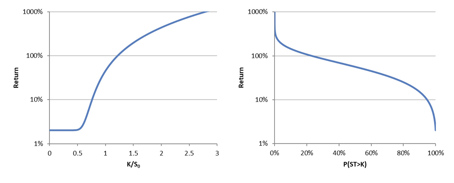
Using an example, assume the expected market return across the stock market is 6% with a standard deviation of 10%, and the risk-free return is 2%. Plotting the return on this bull call strategy (with spread of ) against would produce the graphs shown in Figure 1.
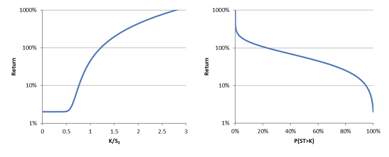
So, looking at the left panel of Figure 1, for a bull call spread strategy with a strike price of less than about 50% of the current stock value, you can be virtually guaranteed a profit and therefore expect to get the risk-free rate. For a bull call spread strategy with a strike price well above the current stock price, there are very high expected returns, but there is also a much higher probability of making a loss.
Looking at the right panel of Figure 1, if the probability of winning is less than ~20%, returns should be expected to be above 100%. If the probability of winning is greater than ~95%, returns should be less than 10%.
This approach is a form of spectral pricing, where the overall investment stock risk is broken down into units, or tranches, of risk. Some units are virtually risk-free, with low returns and low volatility. Others are high risk and high volatility. Given this risk/return profile, if presented with another stock with higher or lower volatility, the aggregate equivalent return can be implied. To do this, the expected return formula needs to be restated as follows:
Note that the denominator of this formula is consistent with the Wang transform but has been independently derived.
Effectively, this approach is doing the same as what the CAPM would do. Given a risk-free rate, and the returns on one stock, the equivalent returns on a second stock (or asset/liability) can be calculated.
5. A clarification of the return parameter
Stock returns are often assumed to follow a normal distribution and to be continuously compounded, which translates to the stock prices following a lognormal distribution. The definition of the return parameter is typically done using generalized Brownian motion and Itô’s lemma, which states
dG=(μ−σ22)dt+σdz.
This is equivalent to
ln(StSt−1)∼normal(μT−σ22T, σ2T).
On the other hand, when we define a normal, or lognormal, distribution, the parameter is also conventionally used to define the first parameter, which has no doubt been a source of confusion to many, when looking at the preceding formula. In this paper, an important distinction is made between the two symbols using So, we can define returns on stocks as
ln(StSt−1)∼normal(˜μT, σ2T).
In practice, to calculate the and from historical data, we would take the following steps:
(i) ˜μ= 1nn∑i=1ln(StSt−1).
(ii) ˜σ2= 1n−1n∑i=1([ln(StSt−1)−˜μ]2).
(iii) μ=˜μ+0.5˜σ2.
6. Comparison to CAPM/Wang
The CAPM formula was introduced in the 1960s, and it remains popular to this day for estimating the returns on an asset class relative to a market portfolio. The formula is where is the expected return on a capital asset. If you were like me, you might have assumed that = but using the methodology outlined in the prior section, it can be shown that the correct formula is = hence the importance of defining the parameter
The Wang transform, developed in 2000 by Shaun Wang, uses a distortion function to price risk—assets or liabilities. When applied to stock pricing it is defined as
F∗(x)=Φ[Φ−1(F(x))+ λ], where λ=(E[Ri]−rf)/σi,
which is consistent with the market price of risk in the classic CAPM. As mentioned in the previous section, the resulting formula for the expected return for the binary gamble incorporates the Wang transform in the denominator, though the Wang transform itself was not used in the derivation, only Black Scholes.
7. Conclusions and further thoughts
This spectral pricing approach is particularly well suited for evaluating systemic market (beta) risk, as it aligns with the market price of risk found in classic CAPM models. However, it does not directly capture additional returns that may arise from alpha risk—that is, asset-specific or liability-specific factors independent of market movements. For example, investments such as catastrophe bonds, which exhibit low correlation with market risk but high volatility, may require a different risk/return framework.
Despite these limitations, the approach remains valuable when the objective is to determine the equivalent return for an asset or liability relative to a reference lognormally distributed asset or liability. This holds true even if the target asset or liability itself does not follow a lognormal distribution.
Furthermore, spectral pricing can be used to allocate aggregate profit across segments of a portfolio. By adjusting model parameters, actuaries can tailor the approach to reflect the risk appetite of a company’s management team, while maintaining a consistent mathematical framework for pricing and capital allocation.